Assessing the RCP / SSP Framework for Financial Decision Making

• The SSP/RCP framework is a powerful construct which has been central to how policymakers develop mitigation strategies and which has been embraced by financial community.
• However, we believe that the scenarios which are developed using a series of models should be subject to scrutiny using well established model risk management approaches.
• Specifically, the framework is deliberately built as a set of scenarios with no associated probabilities, which is challenging for investors to use meaningfully with no view as to likelihood, dispersion and risks around the single paths.
• We highlight areas where the design might lead to an underestimation of the risk, potentially giving rise to a false sense of security on the impacts of climate change and how transition might unfold.

 

1. Introduction

Climate scenario analysis serves as a vital tool for financial institutions (e.g., banks and asset managers) and central banks to assess the risks and opportunities presented by climate change. Typically, climate risk is classed as being either physical (e.g., damage to infrastructure) or transitional (a greater likelihood of, for example, stranded assets or of sovereign defaults with potential financial contagion risk as we move to a low carbon economy). Financial institutions have begun to use scenario analyses to inform client pricing, business planning and internal risk management decisions; central banks have also used them to inform sector-level macro-prudential policies. To align their assessments of forward-looking climate-related financial risks, these actors seek standardised approaches. Traditional financial risk management hinges on making use of relatively rich pre-existing historical data (such as market prices and macroeconomic indicators) in designing tail-risk scenarios. Coupled with the use of appropriate sampling techniques, it is relatively straightforward to generate a large number of scenarios with an associated likelihood, enabling both risk-based asset pricing and estimating quantiles of potential losses to inform capital estimates. For stress tests, a stress situation is created as an exogenous shock to the system, with a given likelihood of occurrence which tests the resilience of a given business line or indeed the entire financial system.

Climate risks are, however, different to financial risks in several ways, and this introduces its own challenges. For physical risks, despite significant research efforts, there are still deep uncertainties associated with the effects of greenhouse gas (GHG) emissions on future economic output. The risks associated with the transition are far more complex than classical financial risk, as they apply not only to the financial system but potentially imply unprecedented structural changes across economies and also involve complex socio-economic feedbacks. It is also clear that markets are not yet able to efficiently process climate information and therefore don’t reflect risks in asset prices accurately. Developing, for example, a probability distribution from past shocks is very unlikely to yield meaningful estimates of future impacts.

Faced with such complexity, firms turn to scenario analysis. However, while financial institutions are uniquely placed to manage financial risks, understanding climate risks necessitates using pre-existing expertise spanning various non-financial disciplines. The Intergovernmental Panel on Climate Change (IPCC) stands as the foremost scientific authority on climate change, tasked with furnishing governments at all levels with scientific information that they can use to understand risks and formulate appropriate mitigatory policies. Unsurprisingly the financial sector has looked to use the high-quality IPCC output.

In Section 2, we give an introduction to how the IPCC scenarios are constructed. We will see how this framework, developed over much of the previous decade, is designed specifically as a scenario planning tool, primarily for the benefit of policymakers. However, it has proven very successful and now ensures consistency across a large body of climate research. In Section 3, we will explore some of the issues associated with this framework, particularly when applied to a financial context. We make some general recommendations as to how to address these risks in Section 4.

 

2. The RCP / SSP framework
 

2.1 Background

Scenarios made their debut in climate research approximately 30 years ago with the first IPCC Assessment Reports (ARs). Their popularity partly stems from the multifaceted nature of climate risk which means that research communities representing different disciplines often focus on particular pieces of the climate crisis aligning with their expertise. Scenarios then represent a means to meaningfully integrate these disparate facets enabling, for example, policy making. This mirrors the challenge faced by financial institutions, discussed earlier.

In order to develop climate scenarios, we might envisage a process similar to that illustrated on Panel A of Figure 1. Indeed, the initial IPCC ARs reflected this structure with the contributions of these research communities accorded to three different working groups (WGs):

• Physical climate analysis is performed by researchers in IPCC WG I. Using emission scenarios as inputs, large scale models project climate (e.g., temperature and precipitation) both regionally and worldwide.
• IPCC WG II assesses the potential impact of climate change on regional and global scales, with specific modelling of particular sectors or biomes. Climate-model projections (as produced e.g., by researchers in WGI) as well as the amount of GHG emissions (as produced e.g., by researchers in WGIII) are inputs to this process.​
• Emissions scenarios are the focus of researchers in WGIII and are generated using process-based integrated assessment models (IAMs). Process-based IAMs are sophisticated constructs that explicitly model the evolution of global energy supply and demand as well as land-use over a long horizon (e.g., until 2100). They have a high degree of detail, particularly for energy supply and demand; these are modelled as a function of underlying socio-economic processes (such as growth in population, development, urbanisation and technology)[1]. In line with the IPCC’s objectives, their principal use is to project cost-effective ‘optimal’ mitigation pathways conforming to stated policy outcomes (e.g., limiting global warming to 2°C). This is achieved by firstly simulating energy demand (from e.g., industry, buildings, agriculture etc). They also incorporate a granular and extensive range of supply options (e.g., wind, solar, nuclear), their costs and how these costs evolve as a result of, for instance, feedback of current/future demand on supply, availability of reserves and learning-by-doing. The lowest cost supply of energy, consistent with matching demand and complying with the stated policy objective, is then determined using an optimisation at each time. This then gives rise to a ’transition’ pathway.

This suggests a sequential relationship between creating emission scenarios, climate projections, and impact studies (Figure 1, Panel A), and indeed this is how the IPCC used to operate. However, this led to a number of issues. The IPCC ARs are produced periodically with the sixth round appearing in 2022. Coordination issues arose because, for example, while impact researchers were applying climate projections to update quantifications of future climate change impacts, physical climate researchers had already moved on to develop the next generation of modelling approaches. This led to a scenario misalignment in the research communities, which complicated the preparation of IPCC ARs. Concerns emerged about potential internal inconsistencies because there were multiple vintages of climate or damage models.

 

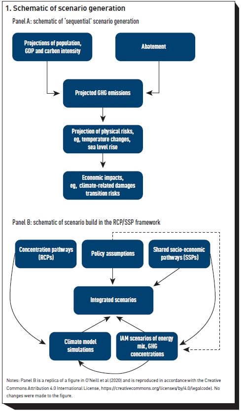
Conceptually also a sequential model feels inappropriate. Future climate depends on energy usage, which in turn depends on socio-economic development and separately on the amount of mitigation (i.e., the extent to which transition to a low carbon economy is expected to happen).

To resolve these issues, a number of IPCC aligned academic research groups developed the so-called Shared Socio-economic Pathway (SSP)–Representative Concentration Pathway (RCP) framework since 2010. In what follows, we discuss the two key constituents before describing how they are combined to give rise to the current IPCC scenario framework, schematically illustrated in Figure 1, Panel B.

 

2.2 The Shared Socio-economic Pathways (SSP)

The SSPs are a small but diverse collection of five pathways designed to provide a common frame of reference across a large range of scenario-driven studies. Finalised versions were released in 2017. These pathways project a range of societal and economic factors including, for example, population, development indicators such as health and education, economic growth, governance paradigms and technological progress. Most factors are given as broad-brush narratives describing changes for large world regions; a subset – population, GDP, urbanisation and educational attainment – are given as quantitative, country-specific projections. This is by design: quantitative estimates are important given their common use as inputs to emissions/climate damages models; furthermore, these variables are strongly inter-related and joint projection is important to ensure scenario consistency. Female education, for example, is seen as a key determinant in projecting both population and GDP. The SSPs do not, by design, include the impacts of climate change or indeed the mitigation and adaptation responses themselves.

The five storylines – SSP1 (sustainability), SSP2 (middle of the road), SSP3 (regional rivalry), SSP4 (inequality), and SSP5 (fossil-fuelled development) – span a spectrum of outcomes related to the ease with which we might manage future climate change. SSPs 1 and 5 envisage relatively optimistic trends for human development and economic growth, arising from investments in education and health, the presence of well-functioning institutions. SSP5 assumes this arises from an energy intensive, fossil- based economy, while in SSP1 there is an increasing shift toward sustainable practices. Conversely, SSPs 3 and 4 describe more pessimistic development trends, with less investment in education or health, rapidly growing populations, and increasing inequality. In SSP3 countries prioritise regional security, whereas in SSP4 large inequalities within and across countries dominate, in both cases leading to societies that are highly vulnerable to climate change. SSP2 envisions a central pathway in which trends continue their historical patterns without substantial deviations. In SSP1 investment in transition leads to positive economic growth, conversely along other pathways transitioning represents a drag on growth.

 

2.3 The Representative Concentration Pathway (RCP)

The Representative Concentration Pathway (RCP) is a greenhouse gas concentration trajectory adopted by the IPCC. Four such pathways were initially used for climate modelling for the IPCC AR5 in 2014. The pathways describe different climate change scenarios, all of which are considered possible depending on the amount of greenhouse gases (GHG) emitted in the years to come. The RCPs – originally RCP 2.6, RCP 4.5, RCP 6.0, and RCP 8.5 – are labelled by the amount of radiative forcing in the year 2100 (2.6, 4.5, 6.0, and 8.5 W/m² , respectively). Radiative forcing, in turn, is a measure of the combined effect of greenhouse gases, aerosols and other factors that cause the trapping of additional heat. The higher values imply higher atmospheric GHG concentrations and hence higher global temperatures[2] as well as more pronounced climate change.

The RCPs were introduced primarily for the benefit of (physical) climate modellers who have different requirements in future emission scenarios than, say, energy system modellers. They want outcomes that cover a wide range of potential future GHG concentrations, allowing the effective evaluation of model behaviour. Hence, while the pathways were developed as outputs of (pre 2010) IAMs, some are extreme and the possibility of such pathways depends strongly on future human development.

 

2.4 Combining the SSP and RCP to generate scenarios

The SSP–RCP framework develops climate and societal futures in parallel, independently of one another and then combine them to create an integrated scenario. Both the SSPs and RCPs by themselves are therefore incomplete by design.

Integration to give a scenario is carried out using the process based IAMs discussed above. IAMs expand the given SSP narrative by elaborating on implications for energy systems, land use changes and quantifying resulting greenhouse gas emissions and atmospheric concentrations. Typically, both ’baseline’ scenarios (future developments assuming no further climate change impacts or new climate policies beyond those currently in place), and ’mitigation’ scenarios (these explore the implications of climate change mitigation policies applied to the baseline scenarios) are developed. Mitigation scenarios are characterised by the level of actions required to reach a given RCP (i.e., level of forcing) by 2100. Multiple different IAMs are used for the quantification of the SSP scenarios; again this is part of the approach by the IPCC recognising that modelling future energy costs is uncertain and subject to model risk.

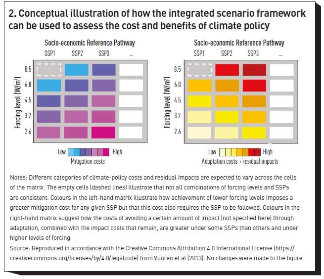
This naturally leads to a matrix of scenarios as illustrated in Figure 2. Each column corresponds to a given SSP, while each row contains climate model simulations based on a forcing pathway. While some combinations of social pathway and forcing are inconsistent with one another (e.g., the narrative in SSP1 is inconsistent with the forcing of RCP8.5), different combinations of forcing and social narrative are consistent, dependent on levels of mitigation[3].

As is standard within the scenario planning literature, there are no probabilities associated with any of the individual scenarios. They were specifically designed as a planning tool and therefore aim to expose a wide range of different ‘plausible’ outcomes; theoretically, all scenarios should be considered equally likely and appropriate actions taken. Probabilities were deliberately avoided as it was felt that they can distract from the story-telling qualities of scenarios, as well as leading to a presumption of predictive accuracy.

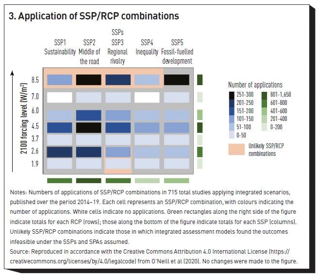
Notes: Numbers of applications of SSP–RCP combinations in 715 total studies applying integrated scenarios, published over the period 2014–2019. Each cell represents an SSP–RCP combination, with colours indicating the number of applications. White cells indicate no applications. Green rectangles along the right side of the figure indicate totals for each RCP (rows); those along the bottom of the figure indicate totals for each SSP (columns). Unlikely SSP–RCP combinations indicate those in which integrated assessment models found the outcomes infeasible under the SSPs and SPAs assumed.

 

2.5 Success of SSP/RCP framework

This framework has proven to be incredibly successful in supporting consistent research across a wide range of topic areas. More than 1,400 analyses using the SSP/RCPs have been published over the past seven or so years. These have covered climate change impacts on a range of sectors (including e.g., air pollution, health, water, forest management, conflict, asset pricing) and future mitigation (e.g., energy transition pathways), adaptation (of buildings, health and water systems).

O’Neill et al. (2020) have conducted a meta-analysis of these studies. They find that the full range of societal and forcing outcomes described in the SSP and RCP frameworks have been explored; we reproduce Figure 3 from their work, which shows an extensive number of studies considering both the risks and the response options for each SSP/RCP combination.

The use of individual SSP/RCP scenarios, however, is somewhat uneven; for example, and there are more studies based on the ’middle-of-the-road’ development pathway (SSP2, 30%) than for the other SSPs. However, the focus on other SSPs and RCPs suggests that these futures are all seen to be worthy of concern. We also note a particular concentration of research associated with the highest forcing pathway RCP8.5. Many have questioned the use of this forcing pathway (Hausfather, 2019), largely because it is unlikely unless we follow a socio-economic narrative analogous to fossil fuelled development; its application in research associated with e.g., SSP2 represents a misapplication, with impacts which are perhaps more sensational than plausible[4].

 

3. Issues

The widespread acceptance of the RCP-SSP scenario framework in the climate change literature has seen its adoption in finance. One of the most prominent examples are the NGFS scenarios (NGFS et al., 2023), for which all economic presumptions stem from the "middle-of-the-road" SSP2 development pathway. This paradigm significantly informs stress tests conducted by major banks; Anecdotally, we also understand the NGFS scenarios are being used for incorporating climate risks into the valuation of long-dated assets.

We argue, however, that while the SSP/RCP framework is well designed, it is important to recognise that the scenarios are outputs from a (relatively complex and somewhat opaque) model infrastructure. The extent to which they are applicable to a given use case (e.g., asset pricing, stress testing) should be carefully validated, ideally using the well-established techniques associated with model risk management. In this section we will discuss some high-level areas where we believe that the use of the SSP/RCP framework should be treated with some caution.

 

3.1 Probabilistic Scenarios and Population Growth

The guiding principle of the RCP/SSP scenarios is that there is no associated likelihood and all should be treated equally; the reality, however, is that some are more equal than others — for example, SSP2-4.5 is the base case favoured by the NGFS (NGFS et al., 2023); conversely with the exception perhaps of SSP5-8.5, most would argue that an RCP of is very unlikely and should not be considered (Hausfather, 2019). This implies a subjective association of probabilities.

We argue that using probabilistic methods (e.g., by building benchmark models based on econometric methods) is a critical tool for challenging the plausibility of scenarios. Probabilistic approaches also enable the development of sensitivities and therefore facilitate decision making on the basis of risks. Separately, reviewing the models underlying the scenario stories - where, for example, common assumptions are used - is also critical, as it may highlight areas where the scenarios are less diverse than we might expect. We are not necessarily advocating the replacement of the SSP/RCP framework, rather that the use of probabilistic methods forms a complementary approach, critical for challenging scenario veracity, enabling greater precision in decision making.

 

 

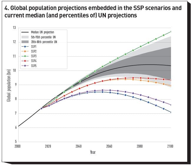
Future population trajectories are critical to the future development narrative underpinning the SSP-RCP framework; smaller populations (all else being equal) lead to reduced GHG emissions. In this section we explore how probabilistic analysis enables greater challenge of these projections; we will highlight that four of the five SSP projections have end-of-century populations below the 20th percentile of current UN projections.

Indeed, up until 2010 most analysis of long-term population was conducted using scenario analysis or by expert judgement specifying future birth and death rates. It is only relatively recently that researchers have begun to apply probabilistic techniques. We reference the work of Raftery and Ševčı́ková (2023) for a review in particular; they have developed Bayesian models for statistically projecting the three components of population change: fertility, mortality and migration on a country-by-country basis. This approach – being probabilistic – enables the generation of country level population projections, age structure, profiles by sex as well as confidence intervals and importantly sensitivities to underlying assumptions; it now underpins the UN’s forecasts.

In Figure 4, we compare the median as well as (5%, 20%, 80%, 95%) confidence intervals against the SSP forecasts for global population. We see that the SSP encompass a greater range for end of century populations; furthermore, that population predictions are generally lower in the SSP, signifying a more rapid fertility transition and greater development than suggested by the work of Raftery and Ševčı́ková (2023). We do not opine on which is more correct; however, we note that the SSP/RCP analysis suggests a generally more positive outlook on development, which has implications for long term economic progress and asset prices. Understanding these sensitivities should therefore form a key part of any assessment prior to adopting this framework.

 

3.2 GDP Projections under SSP framework

Future GDP per capita is a very important indicator of human development and a key determinant of future ability to respond to climate change. GDP (both globally and on a regional/national basis) will also determine asset valuations. In this section, we discuss how GDP projections are developed and benchmark against historical time series. We find:

• Global growth rates are consistent with recent historical observations.
• The determinants of GDP growth are almost certainly more diverse than the ‘human capital’ mechanism which drives scenario growth.
• Empirical GDP growth rates of countries are far more volatile and less correlated than those developed in scenario; not capturing this could impact predictions of economic behaviours such as national savings rates and capital investment.

 

3.2.1 Background

Three alternative projections are available within the SSP framework; nonetheless, each adheres to a common framework, utilising the augmented Solow growth model[5] to project future economic growth. The principal idea behind the model is the so called ’convergence’ mechanism, which posits that as economies advance, the incremental benefits derived from investments decrease. As a result, less developed societies discover it economically advantageous to embrace innovations from the established technological frontier rather than spearhead new technology or methodologies. The enhanced model takes into account human capital, implying that the rate of convergence is influenced by factors such as education levels.

A useful approach to assess the SSP projections is to benchmark against history. Various global institutions (e.g., the World Bank, the OECD and IMF) as well as research groups - the Penn World Tables (PWT) produced by the Potsdam Institute have assembled time series of global GDP data sets (Feenstra, Inklaar and Timmer 2015); most of these provide a comprehensive view across space but data quality is poor prior to the 1960s. We focus on the PWT data.

 

 

3.2.2 Growth Rates

 

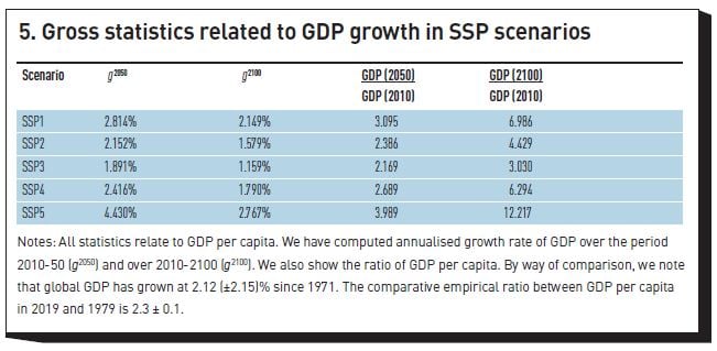
In Figure 5, we have tabulated the average (across the three different models) of annualised growth rates of projected GDP implied by the various SSPs for the period from 2010 to 2050 and 2010 to 2100; we also show the normalised GDP at these two horizons for the five different pathways. We have compared these with the empirically observed growth in GDP obtained from the PWT purchasing power parity data. We find that the projected GDP growth until 2050 in SSP2 matches well what has been observed empirically. SSP1, SSP4 and SSP5 show higher growth, while SSP3 shows reduced growth. Hence to first order the scenarios and SSP2 in particular appear to be calibrated to historical expectations.

The modelled GDP growth rates are found to be significantly higher initially (3.5-4%) and then decline smoothly: growth rates averaged between 2010 and 2100 are markedly lower than between 2010 and 2050. Even in the worst case, we are expected to be twice as rich in 2050 compared to 2010. This is a consequence of the Solow model, whereby the pace of ‘technological’ reform is believed to be decaying. By way of comparison the empirical GDP growth rate (2.12%) is far more noisy, with a standard deviation of ~2%. Empirically there is no obvious evidence of a secular decline.

 

3.2.3 Volatility and Correlation

 

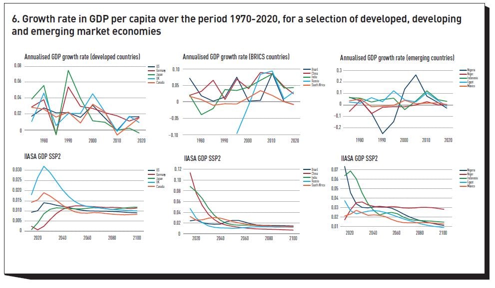
In Figure 6, we compare the GDP per capita growth rates for a set of developed, BRICS and emerging market economies using empirical data with the forecasts for the same countries assuming the SSP2 (middle of the road) scenario.

Two features are immediately apparent in the empirical data: annual growth rates for developed countries are generally smaller than for developing countries; secondly the volatility of growth rates is significant for all countries but is much larger for less developed countries. The projected growth rates are qualitatively different: there is no associated volatility and instead the growth rates show ‘mean reversion’, starting from comparatively high levels; again, the growth rates for poorer countries are much larger than for wealthy nations. The absence of volatility in the projected growth rates leads to them being highly co-integrated.

The absence of volatility reflects the fact that the SSP narratives do not model intermittent growth disruptions arising, for example, from political instability, conflict, commodity price shocks and distortionary fiscal policies. It is of course very challenging to do this. However, it is important to recognise the presence of such effects – because the volatility in growth will lead to (precautionary) savings and differing investment behaviour. Trade flows between countries will also be qualitatively different.

 

3.2.4 Convergence

If convergence significantly influences growth, we should see a consistent reduction in the income disparity between developed and developing nations over time, assuming an upward trend in education levels within developing countries’ populations. Consequently, we should expect that poorer countries would grow far more quickly than developed countries i.e., if we plot the period changes in GDP as a function of GDP, one should expect to see a strong negative slope (Buhaug and Vestby, 2019).

In the left-hand panel of Figure 7, we have plotted a histogram of five-year growth as a function of log GDP per capita for all countries using historical data from the PWT over the period 1970-2020. The right hand panel shows a similar plot except now we plot changes over a 50-year horizon — we illustrate the average of the yearly growth rates since 1970 against log GDP as of 1970 (following Buhaug and Vestby, 2019). In Figure 8, we have plotted comparable data using the SSP projections supplied by the IIASA.

 

 

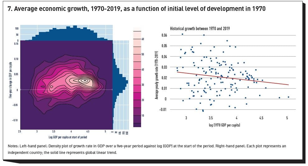
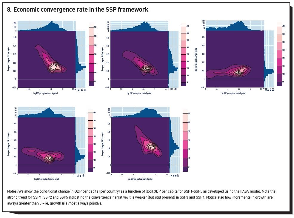
Hence, while there is little empirical evidence of convergence on short horizons, we identify some convergence in the data from the past 50 years; poor countries have grown (on average) (slightly) faster than richer countries[6]. Once again, we also see that growth rates for poorer countries are far more volatile. However, when we examine the SSP projections, the convergence narrative (see Figure 8) is far more marked, and is observable even when we consider five-year changes for SSP1, 2, 4 and 5. Indeed it is only really SSP3 which behaves anything like what has been observed.

Convergence arises in the SSP scenarios because of increased human capital arising from better education. This is perhaps overly simplistic, and means the scenarios are perhaps less diverse than we might like.

The convergence/development narrative is central to the SSP framework. Low/Lower-middle income countries accounted for 13% of global GDP in 2010 but are expected to account for to 22-29% (32-49%) by 2050 (2100). Even ’within model’, such growth may prove unrealistic, because the scenarios do not incorporate climate feedbacks. A number of authors have highlighted through econometric methods that climate change impacts the growth rate of GDP of poorer countries. Basic calculations suggest that climate damages could markedly reduce GDP growth in these countries leading to the persistence of global inequality.

Furthermore, there is a lag before improvements in human capital translate into higher economic growth; similarly, such changes must also be accompanied by other measures such as institutional reform, diversification away from reliance on extractive industries etc, all of which require time. This lag is not factored into the narratives.

Better education and higher GDP per capita are likely to lead to a more rapid fertility transition, which in turn implies a lower population, as seen in Figure 4. Hence it seems that:

• The scenarios project significant reductions in inequality and growth in GDP in the first part of the century. This may bias towards a strategy of delaying climate action as we will be wealthier and therefore better placed to finance mitigation subsequently.
• The scenarios are not as pessimistic as one might generally consider when conducting stress testing.

 

3.3 Discounting

The discount factor chosen plays a critical role in shaping the course of action within models determining tradeoffs between actions now and those in the future. In this section, we will discuss how the discount factor in the IPCC framework is related to the trade off in timing of abating GHG emissions in process based IAMs. This choice of a discount curve, however, has very wide-reaching implications on the transition pathway (and for subsequent scenario expansions such as for asset pricing); in what follows, we highlight some of these and how one might challenge the resulting narrative.

 

3.4 Discounting in Process Based IAMs

Assuming there is no natural decay of CO₂ in the atmosphere[7], abating one ton of CO₂ today is equivalent to abating the same amount in the future. The growth of the (expected) carbon price should then be equal to the risk adjusted discount rate; in the case where there is no uncertainty (e.g., in economic output or future cost evolutions) then we would expect that the growth rate of carbon prices (g) should be equal to the risk-free interest rate ( ) i.e.,                                                                                                                                                                      

This result is easily generalised to the case where we allow for decay of greenhouse gases in the atmosphere and we allow for uncertainty (Gollier 2021):

                                                                                                                                                                

where is the rate of natural decay of greenhouse gases in the atmosphere, and  represents the abatement risk premium and is the product of the income-elasticity of marginal abatement cost and the aggregate risk premium  in the economy. Following Gollier (2021), we have developed the annual discount rate (or equivalently the growth in carbon price) within the process based IAMs, finding a median value of 5%, although in certain scenarios the growth rate can be as high as 15%. By way of comparison, Gollier has examined the rate of growth of the social cost of carbon in an extended cost benefit IAM[8] which incorporates uncertainties in economic progress and technological development, and following on from Equation 2 obtains a value of 3.5%, with approximately half of this arising from the impact of uncertainty. Separately Tol (2022) has surveyed the academic literature for the growth rate of the social cost of carbon in such models and highlights a range between 1.5% and 3%, assuming approximate calibration to market interest rates. These relatively small changes in discount factor lead to very significant differences in abatement expenditure in the future (a factor of 2-3 by 2050 and 4-10 by 2100).

 

3.4.1 Intergenerational Equity and Asset Pricing

Discounting has direct consequences for inter-generational equity: high values of the discount rate reduce the mitigation effort of current generations deferring it to the future. This raises ethical issues, especially because future generations will also be the ones bearing the majority of the impacts of climate change. Indeed, a frequent criticism of the DICE model (Nordhaus 2017) is that the chosen discount factor (at 1.5%!), calibrated to market discount factors, is too high and is ethically unfair.

Gollier argues on the basis of his results that the SSP/RCP framework of the IPCC inefficiently allocates abatement efforts over time. The same final concentration of GHG in the atmosphere could be obtained with a smaller impact on inter-generational welfare by abating more today (and hence a higher expenditure today) and abating less in the future[9]. The choice of discount factor assumed implicitly incentivises ‘waiting’. He points out that this is because process based IAMs do not find, by design, the temporally optimal strategy.

 

3.4.2 Impact of Discounting on Technology

The choice of discount rate plays an important role in determining future technological pathways. As investment in abatement is, relatively speaking, delayed there is a greater probability that we will need to use carbon dioxide removal technologies to attain the end of century greenhouse gas concentrations i.e., we will overshoot the carbon budget. This is the principal reason why the optimisation approach within the IAMs leads to the extensive adoption of BECCS (Bioenergy with Carbon Capture and Storage); this is somewhat at odds with expert views. We also highlight the focus by a number of sources on removal technologies such as direct air capture, which may again be overly optimistic.

The use of an inappropriate discount rate may therefore bias policy makers and potentially investors.

 

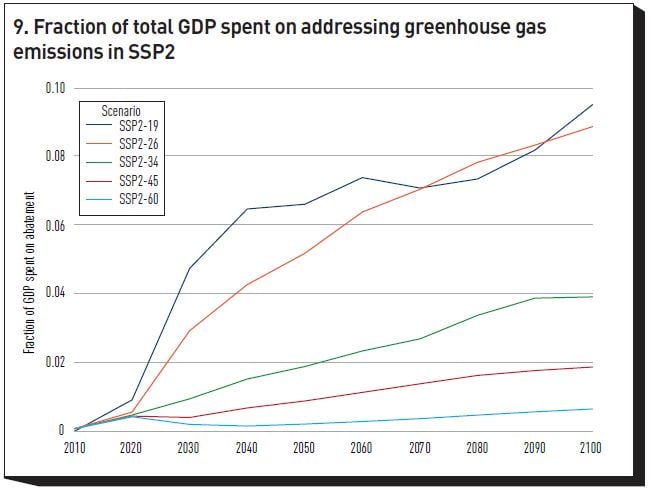
3.4.3 Future Growth of Expenditure on Abatement (Carbon Tax)

The SSP/RCP datasets detail future taxation on GHG emissions; we plot this for SSP2 in Figure 9. As expected, we find that the carbon tax increases rapidly as we entertain more restrictive forcing scenarios, rising for example to 8% of global GDP for SSP2-26. The rapid increase is a direct consequence of the discount rate chosen in the IPCC scenarios. Indeed, for SSP3 taxation levels need to exceed total GDP to achieve low temperature anomalies.

 

 

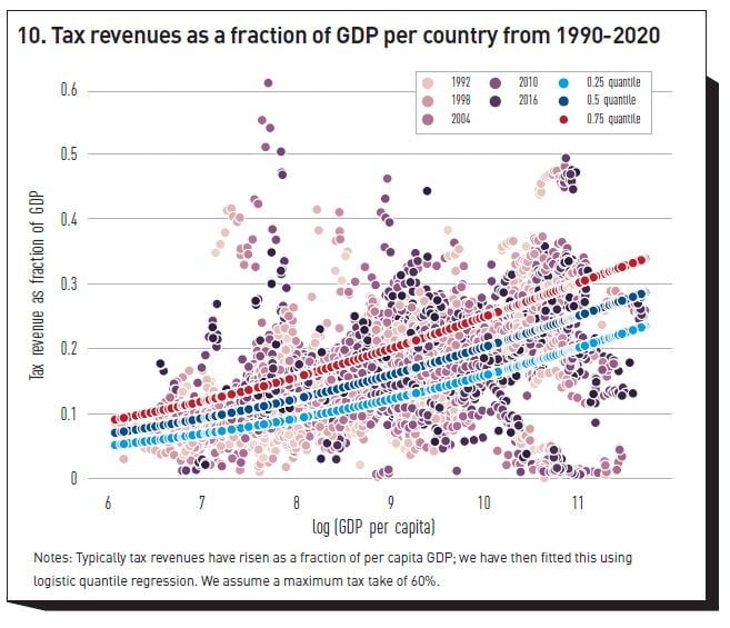
As discussed in 2.3, the levels of taxation are assumed to be exogenous, determined by optimisation and hence enable the SSP/RCP matrix. To explore this further, we have analysed taxation as a function of GDP per capita, and, as per other studies in the literature (Le, Moreno-Dodson and Bayraktar, 2012), we find a strong relationship (see Figure 10).

 

We characterise this behaviour using a logistic function assuming maximal taxation of 60%:

                                                                                             

and have then parameterised on the basis of national GDP and taxation over the past 30 years (see Figure 9).

This model assumes that the ability to increase taxation depends on increasing GDP per capita. For example, we find that the change in taxation assumed in SSP2 to achieve RCP1.9 requires spending an additional ~4% of global GDP on abating the effects of climate change. We estimate that this requires ~28% increase in GDP per capita which is challenging to achieve from a growth perspective in SSP2 (see Figure 5). This also assumes that all benefits of increased taxation would be diverted solely to fighting climate change, which is of course extremely unlikely. We argue that analysis of taxation patters is a useful approach for benchmarking the likelihood of particular transition scenarios.

 

3.5 Asset Pricing

Lastly we consider the pricing of assets using the SSP/RCP scenarios.

The fundamental theorem of asset pricing states that the price of any asset is its expected discounted payoff. Suppose we have an asset, worth  at time t. Assume that the asset pays a dividend in the next period, . Then the fundamental theorem states that:

                                                                                                               

where  is the so-called stochastic discount factor (sdf) over the period (t, t+1). When computing the expectation in Equation 4, we probability weight over all possible future states of the world. Furthermore how anticipated future payoffs are evaluated depends on statistical properties of the sdf and how it correlates with future cashflows (here the next period’s value and dividend). Thus for example, assets that tend to have good payoffs in bad states of the world will be valued more highly than other assets which, for example, payoff well in good states of the world only. This is because such assets pay well when funds are more urgently wanted.

This means that computing expectations by naively conditioning on a particular SSP / RCP scenario could lead to inaccurate asset valuations, as it implicitly assumes that the likelihood of other states is very small (zero). It is likely that such approaches do not capture the diversification associated with green/brown assets accurately either. Asset pricing likely requires probabilistic scenarios.

 

4. Conclusions

The SSP/RCP framework is a powerful construct which has proven very useful both in harmonising research into climate change and enabling policymakers to develop mitigation strategies on both a global and national scale. Given the level of scientific consensus, it is unsurprising that this framework has been adopted within the financial community. We argue that while scenarios are useful, it is important that additional analysis is undertaken as part of adoption:

• The scenarios are developed using a modelling chain, and as such they should be subject to scrutiny using well established model risk management approaches.
• Specifically while the framework is deliberately built as a scenario matrix, with no associated probabilities, we argue that the use of econometric and probabilistic techniques provide valuable insight. Indeed, we would argue that it is challenging for investors to use the framework meaningfully without enhancements to incorporate a view as to likelihood, dispersion and risks around the single paths in the framework.
• The scenarios focus on transition and hence the social development / energy nexus; when extending to areas such as asset pricing, identifying and consistently modelling key risk drivers will be key.
• Many of the identified issues lead to an underestimation of the risk, potentially giving rise to a false sense of security on the impacts of climate change and how transition might unfold.

 

 

Footnotes

[1] However, future impacts of climate change are generally excluded

[2] Forcings of 2.6, 4.5, 6.0, and 8.5 W/m²  corresponds approximately to temperature anomalies of approximately 1.8, 2.6. 3.3, 4.6°C by 2100.

[3] These scenarios are commonly referred to as SSPx - y, where x is the specific SSP and y represents the forcing pathway, defined by its long-term global average radiative forcing level.

[4] This body of research can therefore be potentially misleading, as the likelihood of e.g., SSP2-8.5 is vanishingly small; however, probabilities are deliberately not part of the framework.

[5] This is a widely used economic development model and generally favoured because of its good empirical fit and connection with microeconomic theory.

[6] We observe a difference of ~1%in annual growth rates on the basis of OLS across countries.

[7] This is not unreasonable for CO₂, but other GHGs such as methane are removed by biochemical processes more rapidly.

[8] These are models such as DICE, which explicitly determine the intertemporally optimal abatement strategy by maximising a social welfare function.

[9] To set against this, proposals for rate of growth of the social cost of carbon in e.g., France and the UK have often exceeded 5% per annum; however, such headline rates disguise current low levels and the fact that schemes often apply only to a subset of emissions.

 

References

Buhaug, H. and J. Vestby (2019). On Growth Projections in the Shared Socioeconomic Pathways. Global Environmental Politics 19(4): 118–32.

Feenstra, R.C., R. Inklaar and M.P. Timmer (2015). The Next Generation of the Penn World Table. American Economic Review 105(10): 3150–82. https://doi.org/10.1257/aer.20130954

Gollier, C. (2021). The Cost-Efficiency Carbon Pricing Puzzle. CEPR Discussion Paper No. 15919. CEPR Press, Paris & London. https://cepr.org/publications/dp15919   

Hausfather, Z. (2019). Explainer: The High-Emissions ‘RCP8. 5’global Warming Scenario. Carbon Brief 21(8): 2019.

Le, T.M., B. Moreno-Dodson and N. Bayraktar (2012). Tax Capacity and Tax Effort: Extended Cross-Country Analysis from 1994 to 2009. World Bank Policy Research Working Paper, no. 6252.

NGFS, PIK, IIASA, UMD, CA, ETHZ and NIESR (2023). NGFS Climate Scenarios: Technical Documentation. https://www.ngfs.net/sites/default/files/media/2023/11/07/ngfs_scenarios...

Nordhaus, W.D. (2017). Revisiting the Social Cost of Carbon. Proceedings of the National Academy of Sciences 114(7): 1518–23.

O’Neill, B.C., T.R. Carter, K. Ebi, P.A. Harrison, E. Kemp-Benedict, K. Kok, E. Kriegler et al. (2020). Achievements and Needs for the Climate Change Scenario Framework. Nature Climate Change 10(12): 1074–84. https://doi.org/10.1038/s41558-020-00952-0

Raftery, A.E. and H. Ševčı́ková (2023). Probabilistic Population Forecasting: Short to Very Long-Term. International Journal of Forecasting 39(1): 73–97. https://doi.org/10.1016/j.ijforecast.2021.09.001

Tol, R.S. J. (2022). Estimates of the Social Cost of Carbon Have Increased over Time. https://arxiv.org/abs/2105.03656

Vuuren, D.P. van, E. Kriegler, B.C. O’Neill, K.L. Ebi, K. Riahi, T.R. Carter, J. Edmonds, et al. (2013). A New Scenario Framework for Climate Change Research: Scenario Matrix Architecture. Climatic Change 122(3): 373–86. https://doi.org/10.1007/s10584-013-0906-1.