Climate shocks or the death by a thousand cuts? The effect of climate change on the valuation of equity assets

Key Fingings

• The uncertainty of climate and economic outcomes and the state dependence of discounting are two key and much neglected contributors to changes in climateaware equity valuation.
• The magnitude of portfolio losses depends on the aggressiveness of emission abatement policy, the presence or otherwise of tipping points, and on the extent of central banks’ willingness and ability to lower rates in states of economic distress.
• Severe impact on equity valuation can be obtained with very plausible combinations of policies and physical outcomes; and there is considerably more downside than upside risk – more than 40% of global equity value is at risk unless decarbonisation efforts accelerate and losses could exceed 50% with near climate tipping points.
• If prompt and robust abatement action is taken, losses can be kept below 10% even in the presence of tipping points.

Rethinking equity valuation in the face of climate change

How large can we expect the impact of physical climate risk on the value of global equities to be? At a very fundamental level, does climate change matter for asset valuation? We look at the impact of climate change on the price of a global equity index, and we show that, for plausible combinations of abatement policies, the impairment on equity values can be large.

Providing an answer to the motivating questions above is of obvious importance to investors. However, policymakers and prudential regulators and asset managers should also be interested. Regulators want to make sure that the portfolios of the institutions under their watch may not become so severely impaired as to cause instability in the financial institutions themselves. For policymakers, equity valuation can be a bellwether of broader economic conditions: avoiding states of severe equity impairment is one indicator of a safe policy course. And as for asset managers, their profitability comes not just from the fees they charge and on the nominal amount of investment they manage, but also on the mark-to-market of their assets under management.
 

Climate risk can affect asset valuations both via the transition-risk and via the physical-risk channels.[1] Transition risk has received more attention than physical risk: for example, the scenarios prepared by the Network for the Greening of the Financial Sector (NGFS) have historically focused on assessing the economic and financial impacts of a (potentially disorderly) shift to a low-carbon economy. Indeed, studies that have tried to detect the impact of physical climate change on asset prices have either concluded that physical climate risk is currently not priced in (but transition risk is – see, eg, Bolton and Kacperczyk [2023]), or, that the effects, while statistically significant, are economically small. But should the effect of physical risk on asset prices really be so negligible? To address this question, we combine tools from the macro-asset pricing literature that examine how long-term macroeconomic uncertainty affects current valuations (Bansal and Yaron [2004]) with an extended version of the Dynamic Integrated Climate-Economy (DICE) model (Nordhaus and Sztorc [2013]), the prototypical model for integrated climate-economic assessment. What we find is that the largest downwards revisions of equity values occur for the least aggressive abatement schedules, ie, when temperatures are allowed to rise to levels for which physical damages become important. To the extent that abatement costs can be thought of as a reasonable proxy for transition costs, our conclusions point to the fact that the highest equity losses are incurred because of physical, not transition, risk. Actually, robust abatement (though costly) can effectively limit the valuation impairment even in the case of a much more severe dependence of damages on temperature than it is currently estimated. Even from a narrow equity valuation perspective, prompt and decisive abatement action represents an insurance premium well worth paying.
 

The approach we follow to estimate the value of global equities has solid theoretical foundations, but is also very intuitive. What the holders of securities receive in the form of dividends is the fraction of what the economy produces that accrues to the providers of capital. The greater the impairment to net economic output due to physical damages and abatement costs, the smaller the future expected dividends. The value of equity stock then comes from discounting back to today these future cashflows – and, as we discuss, this is where state-dependent discounting plays an important role. The only ingredient missing from this thumbnail sketch of our procedure is that equities are a leveraged claim to what the economy produces, and this leverage (as leverage always does) magnifies both the upside and the downside.

One key result of our study is that the state-dependence of climate damage introduces two opposite effects: while climate damages reduce ‘consumption dividends’, they also lower the stochastic discount rate, thereby increasing the present value of these impaired dividends.
The overall impact on valuation is the outcome of this tug of war. 

When we estimate the impact of physical climate risks on the value of a synthetic global equity index using this approach, we find that the effects can be substantial. This is particularly the case in a world with climate tipping points; however, even in the absence of tipping points[2], we estimate a difference in the valuation of global equities with respect to a no-climate-damage world ranging from less than 10% if prompt and robust abatement action is taken, rising to more than 40% in a close-to-no-action case. In the presence of climate tipping points, this range widens from less than 10% for robust abatement to more than 50% in the case of very low abatement. 

As we discuss at greater length below, we find that for equity values to be mildly affected by physical climate risk three conditions must be met:

• an emission-abatement policy much more aggressive than that currently followed should be pursued; 
• the threshold temperatures of tipping points should be located well above the temperatures that we may reach with moderate abatement policies; and 
• monetary authorities should be able and willing to cut rates aggressively in periods of economic distress (of low consumption).
   

None of these conditions is a priori implausible (with the greatest uncertainty surrounding the location and effect of tipping points), but none should be taken for granted. Great uncertainty therefore surrounds the estimation of physical climate impact, with very plausible combinations of policies and physical outcomes producing very severe effects on equity valuations, and with considerably more downside than upside risk.

We present our results by calculating the difference in equity valuations when different abatement policies are implemented and the valuation that would apply in a world in which global warming did not affect the economy, and therefore had no impact on valuation. The latter scenario is useful as a reference point, but hardly realistic. The truly relevant question is to what extent our findings, if correct, are already embedded in the prices of equities. We present indirect  evidence that current equity prices seem to reflect only marginally the effect of climate change – and that, to the modest extent they do, they seem to reflect transition, but not physical risk. If, as we show, the effect of weakly unabated climate change on equity valuation is large, this could give rise to a substantial revaluation. For a fuller discussion of this point, see our section on Key findings.

How we model the impact of climate on global equity valuations
 

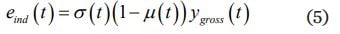
To arrive at the change in the value of equity due to climate change first we have to estimate the future dividends, and then we must discount them. Just as dividends are the fraction of the net revenues of a firm which is not reinvested for future production, so, from the macroeconomic perspective we are taking, consumption (ie, the fraction not channelled into savings/investments) is the ‘dividend’ of the global wealth portfolio, , given by

where denote the time-i state-dependent discount factors and consumption streams. We calculate both these quantities using a much-enriched version of the DICE model (see Rebonato, Kainth and Melin [2024] for a detailed description). In essence, with our approach we account for some of the deep uncertainties inherent to the problem, related to:

• carbon climate dynamics and the presence of tipping points;
• future economic output;
• economic damage functions;
• the pace of future abatement.

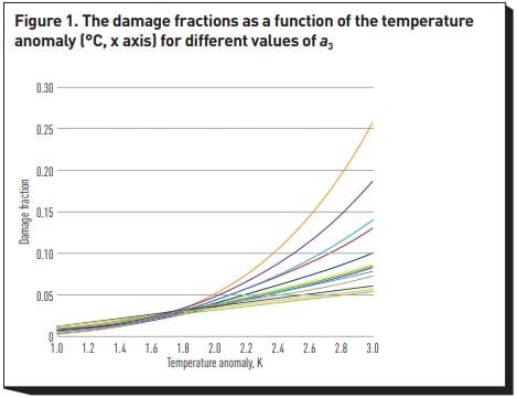
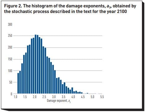
In particular, as customary in the literature, the damage functions, Ω(T), (the function, that is, that relates temperature increases to economic damages) is modelled as

where T denotes the temperature anomaly. There is little agreement in the literature about the value of the damage exponent, , which controls how quickly damages increases with temperature. We therefore centre this value around the consensus estimate from the literature
(see, eg, Nordhaus and Sztorc [2013], Howard and Sterner [2017], Rudik [2020]), but allow for significant dispersion around this value, as shown in figures 1 and 2.

In our study we present results both without and in the presence of tipping points. To model their impact on economic output, we used a simplified approach where damages increase slowly at first, then accelerate around a critical temperature threshold, , and finally level off at a maximum damage level, H. This behaviour is captured by an S-shaped (sigmoid) function, which describes how the fraction of economic output lost increases with rising temperatures:

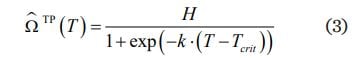
where is the fraction of economic output lost because of tipping pointinduced climate damages, H denotes the maximum damage fraction associated with the tipping point(s), the level at which the damage fraction reaches H/2, and k regulates the speed of ‘ramp-up’. We have chosen H = 0.30, = 2.5 and a speed  The choice of the threshold level, , has been informed by the estimates in the most recent report by the Intergovernmental Panel on Climate Change and in Lenton et al (2008) of its nearest plausible level.

We do not claim that our location for the threshold of the tipping point is the most likely, or that the maximum loss associated with its inset is known with any precision. We simply want to explore what the equity valuation implications would be of a severe but plausible tipping point
specification. Given the large uncertainty surrounding this topic, investors should at the very least have this possibility at the back of their minds – not for nothing, in its comprehensive study of abrupt climate change (NRC [2002]), the National Research Council refers to tipping points as ‘inevitable surprises’.

Another very important component is economic growth: higher economic output in fact gives rise to greater emissions, greater concentrations, higher temperatures and higher damages. We model economic growth using the seminal ‘long-run-risk’ model by Bansal and Yaron
(2004), as adapted to climate change problems by Jensen and Traeger (2014). This model is described in detail in Rebonato, Kainth and Melin (2024). Here we simply recall that this model (when coupled with Epstein and Zin [1989] utility functions) allows the simultaneous recovery of the equity risk premium and of the level of rates. These features make it very suitable for the asset pricing analysis we are interested in.

A last modelling feature that we should discuss is the set of chosen abatement schedules. As we have explained, we consider two sets of cases: an economy without climate change damages and an economy with climate change damages, and different degrees of abatement ‘aggressiveness’. For the latter, the speed of abatement, ie, the emission abatement function, μ(t), is controlled by a single parameter, κ (the abatement speed) in the function

where t denotes time in years from today, and μ0 is today’s (observed) level of abatement.
 

The abatement function, μ(t), is implicitly defined as in Nordhaus and Sztorc (2013) by

where denotes industrial emissions and σ(t) is the time-t emission intensity of the economy (emissions per unit of gross economic output,  We consider in our study five possible values for the abatement speed, κ: 0.001, 0.01, 0.02, 0.03 and 0.04 . 

Clearly, a variety of abatement patterns, much more complex than the simple functions shown in figure 3 can occur in real life, and our choice of four stylised abatement patterns may seem unduly restrictive. However, it is possible to show that the functions μ(t) in equation 4 are actually more general than they at first appear.[3] The decay constant, κ, in equation 4 is therefore a very useful statistic to capture in a synthetic way most of the information embedded in a number of potentially complex abatement schedules.
 

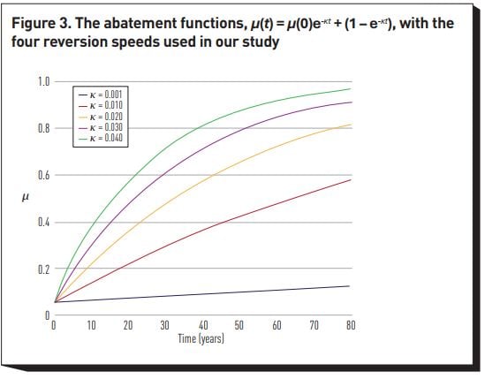
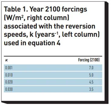
To give an idea of the aggressiveness (or lack thereof) of the abatement schedules we have chosen, the fastest (associated with κ = 0.04) produces average temperature anomalies by the end of the century of about 2°C (just within the upper limit of the Paris Accord range), and implies that the ‘distance’ to full decarbonisation will be halved every 17 years. As for our slowest abatement speed (κ = 0.001) it corresponds to a 2100 forcing (balance of energy in minus energy out) of 7W/m². We recall that a forcing of 8W/m² has been described by Hausfather and Peters (2020) as implausibly high (ie, as implying an excessively slow decarbonisation process), but has been defended by Schwalm, Glendon and Duffy (2020) as being actually consistent with the pace of decarbonisation observed to date. Our values therefore bracket reasonable optimistic and pessimistic scenarios for abatement. Table 1 shows how the abatement speed, μ, in equation 4 can be associated with a degree of forcing. 

Within this framework, the value,  of a global equity stock today can be obtained as the expectation over the discounted payoff:

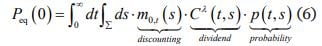
where p(t,s) represents the probability of the state variables being in state s at time t, C(t,s) and are the consumption and discount factor (to time zero) in state s at time t. We then integrate over the whole of the state space (denoted by Σ) and over all times. Despite the forbidding appearance, equation 6 is easy to interpret: the term denotes the discount factor from time t to today (time 0), with the argument s indicating that the magnitude of the discounting depends on the state, s, of the economy; the term  signifies the time and state-dependent ‘dividend’, which is just consumption raised to the exponent, λ, to account for leverage; and, finally, the term p(t,s) denotes the probability of being in state s at time t. The inner integral means, for each time, a sum over all the states, and the outer integral carries out a sum over time. So, equation 6 simply carries out the valuation of a global equity stock along the lines of well-known expected-discounted-cashflow models.

Key findings

Our computational procedure is described in detail in Rebonato, Kainth and Melin (2024), who also carefully identify the contribution to valuation impairment associated with stochasticity in economic growth and uncertainty about the damage exponent. Here we present a more succinct account of the more salient features of that work.

We quantify the change in valuation caused by climate damages by computing the ratio of the equity value with climate damages to the value without climate damages. More precisely, we define the loss ratio as

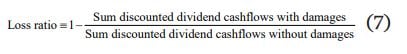
This is the quantity reported in tables 2 and 3 for the no tipping point and tipping point case, respectively. In both tables the number in square brackets show the loss ratio when the discounting is assumed to be non state-dependent. The different rows refer to plausible choices for a key parameter, the elasticity of intertemporal substitution (EIS), of the utility function which is maximised by our chosen model.[4]

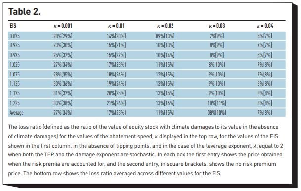
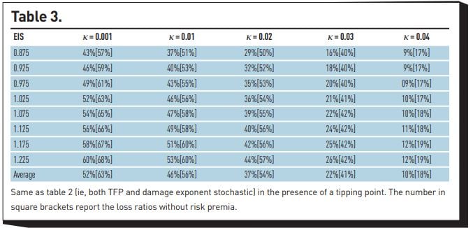
The first observation is that in the case of slow abatement the losses can be large, especially (but not only!) if tipping points are present (see the columns on the left of the two tables). Conversely, the impact even of nearby tipping points on valuation can be mitigated by strong and early action (see the columns on the right of the two tables). Note that a robust and costly abatement can limit the loss ratio to about 10% even if tipping points are as severe and ‘nearby’ as we have assumed.

Second, the fact that the highest loss ratios occur for the lowest abatement schedules implies that physical damages have a far greater impact on equity valuations than abatement (transition) costs. It is usually argued that transition costs may be smaller in absolute value, but, by virtue of being ‘front-loaded’, are discounted less and therefore have a greater valuation impact than the larger but remote physical damages. The infinite-maturity nature of equity assets suggests that this is not necessarily the case, and that the correct discount factor should be a result of a proper analysis, not of our prejudices.

This naturally brings us to the third point, ie, the effect of discounting. We note from the tables that taking stochastic discounting into account reduces the magnitude of the valuation impairment. (Loss ratios in square bracket in the two tables are obtained with the same average discount factor, but after suppressing its state dependence.) This happens because in states of high climate damage consumption growth is reduced, and hence discounting rates, which can be approximately written as

are also reduced. (In equation 8 denote the pure impatience discount rate, the coefficient of risk aversion and consumption growth, respectively.) This dependence of the rate of discounting on the state of the economy is not just a theoretical feature, but finds a parallel in the actions of the monetary authorities that, inflation permitting, tend to lower rates in periods of subdued economic growth (the philosophy underpinning the ‘Greenspan put’). This is the origin of the tug of war between the expectation effect of higher damages, and the discounting effect, which pull in opposite directions.

Key messages for investors

The magnitude of the equity impairment that we have estimated (and which has been obtained with conservative modelling choices) raises the question of the extent to which these effects are already embedded in equity prices. It is difficult to answer this question with certainty. However, as noted in Rebonato (2023), studies of the so-called climate beta (ie, of the sensitivity of prices to climate news) and of the climate risk premium (how much the return of climate-sensitive securities should differ from the riskless rate) have so far yielded either null, or contradictory, or statistically-but-noteconomically significant results. Given the number of studies which have been devoted to the topic, and the inconclusive results that have been obtained, it seems unlikely that equity prices fully embed this information. If our analysis is correct, a substantial aggregate equity repricing could be expected.

What could the timing of this repricing be? It is extremely difficult to see. It is however hard to imagine that either a new climate event or scientific report could shift the current muted embedding of climate risk in asset prices. What is more likely is that the equity losses that we estimate may come about as a series of negative, and individually rather minor, revisions of expected economic results. If this is correct, the eventual equity repricing may come about as the result of a steady negative ‘headwind’. Indeed, many studies (see, eg, Burke, Hsiang, and Miguel [2015], Kotz and Wenz [2021], Bilal and Kaenzig [2024], Park [2024]) suggest that an impairment to productivity, rather than headline-grabbing catastrophic losses, may be the financially most likely channel through which climate change could affect economic output.

In sum, the key messages for investors are:

• From the perspective of a professional investor, our study provides help and suggestions that go beyond the presentation of the range of potential equity losses. One important take-away lesson is the huge uncertainty that surrounds all these estimates. Point estimates (and especially point estimates with many decimal points) are not only foolhardy, but dangerous. After all, whatever one may think of the Black and Litterman (1991) model, one enduring contribution of their approach is that, whatever one’s ‘view’ about the returns to be expected from an asset class, our uncertainty about this view radically changes the optimal allocation.
• The second important message to investors from our work is that the discounting of future cashflows is less straightforward than one often assumes. Rule-of-thumb approaches for discounting future cashflows, such as using a weighted average cost of capital, can work well for the settings for which they have been created, but may not be transportable to the valuation of climate-dependent cashflows. Whether they are or not depends on the specific application, and, as we have seen, the difference can be large. An example that a one-size-fits-all discount factor may not be suitable to all climate change settings is the difference between transition costs and physical damages: the former are probably weakly of the state of the economy; the latter are certainly strongly correlated with it.
• Finally, we note that the central banks’ ability to lower rates in periods of distress (which would normally undergird the equity valuation) may be more limited for the poorer countries, which tend to have little fiscal space. Unfortunately, some of these are exactly the countries that are more likely to be severely affected by climate change.

Footnotes

[1] Broadly speaking, physical risk pertains to the direct impacts on output, capital or economic growth resulting from anthropogenic climate change. Transition risk, on the other hand, encompasses the economic costs incurred during the shift to a low-carbon economy aimed at mitigating future physical risks. These costs can be exacerbated by either a rushed or delayed implementation of mitigation strategies.

[2] Tipping points are critical thresholds in the Earth’s climate system, above which small temperature changes can trigger swift, significant and often irreversible, changes in environmental conditions.

[3] One can show that, under mild assumptions, all abatement functions which have the same emissionweighted average abatement to a given horizon produce the same horizon CO2 concentrations, and hence, given a climate model, the same temperatures.

[4] The elasticity of intertemporal substitution is the inverse of the aversion to uneven consumption. The higher the EIS, the lower this aversion. A lower aversion to uneven consumption means that agents are less disinclined from investing in costly abatement today despite the fact that they expect their descendants to be richer.

References

• Bansal, R., and A. Yaron (2004). Risks for the Long Run: A Potential Resolution of Asset Pricing Puzzles. Journal of Finance 59(4): 1481–1509.
• Bilal, A., and D. R. Kaenzig (2024). The Macroeconomic Impact of Climate Change: Global vs. Local Temperature, NBER working paper no 32450, 29 (2): 1–72.
• Black, F., and R. Litterman (1991). Asset Allocation Combining Investor Views with Market Equilibrium. Journal of Fixed Income 1(2): 7–18. Bolton, P., and M. Kacperczyk (2023). Global Pricing of Carbon-Transition Risk. Climatic Change 78(6): 3677–3754.
• Burke, M., S. M. Hsiang and E. Miguel (2015). Global Non-linear Effect of Temperature on Economic Production. Nature 7577: 235–239.
• Epstein, L. G., and S. E. Zin (1989). Substitution, Risk Aversion, and the Temporal Behavior of Consumption and Asset Returns: A Theoretical Framework. Econometrica 57(4): 937–969.
• Hausfather, Z., and G. P. Peters (2020). Emissions – The Business-As-Usual Story Is Misleading. Nature 577: 618–620.
• Howard, H. P., and T. Sterner (2017). Few and Not So Far Between: A Meta-Analysis of Climate Damage Estimates. Environmental and Resource Economics 68(1): 197–225.
• Jensen, S., and C. Traeger (2014). Optimal Climate Change Mitigation under Long-Term Growth Uncertainty: Stochastic Integrated Assessment and Analytic Findings European Economic Review 69(C): 104–125.
• Kotz, M., and L. Wenz (2021). The Impact of Climate Conditions on Economic Production: Evidence from a Global Panel of Regions. Journal of Environmental Economics and Management 103: 102360.
• Lenton, T. M., H. Held, E. Kriegler, J. W. Hall, W. Lucht, S. Rahmstorf and H. J. Schellnhuber (2008). Tipping elements in the Earth’s climate system. Proceedings of the National Academy of Sciences 105(6): 1786–1793.
• Nordhaus, W. D., and P. Sztorc (2013). DICE 2013R: Introduction and User’s Manual. Yale University, New Haven, Connecticut, US.
• NRC (2002). Abrupt Climate Change: Inevitable Surprises. The National Academies Press, National Research Council.
• Park, R. J. (2024). Slow Burn: The Hidden Cost of a Warming World. Princeton University Press.
• Rebonato, R. (2023). Asleep at the Wheel? The Risk of Sudden Price Adjustments for Climate Risk. The Journal of Portfolio Management 50(2): 20–57.
• Rebonato, R., D. Kainth and L. Melin (2024). The Impact of Physical Climate Risk on Global Equity Valuations. Environmental and Resource Economics forthcoming: 1– 34.
• Rudik, I. (2020): Optimal Climate Policy when Damages Are Unknown. American Economic Journal: Economic Policy 12(2): 340–373.
• Schwalm, C. R., S. Glendon and P. B. Duffy (2020): RCP8.5 Tracks Cumulative CO2 Emissions. Proceedings National Academy of Science 117(33): 19656–19657