Commodities, Crude Oil, and Diversified Portfolios

With concerns on inflation flaring up, there has been renewed interest in potentially including commodities in diversified portfolios.  This article will build off prior research in examining which commodities to include and in what size.  After briefly reviewing the relevant literature, we will propose a novel and uncomplicated portfolio solution, which takes into consideration both historical results and plausible new paradigms.  In addition, an investor would be able to implement this portfolio solution through deeply liquid futures markets.

 

Literature Review

Commodities for Inflation-Hedging

Neville et al. (2021) provides an updated look into inflation hedges with a long-term dataset of monthly commodity futures prices from 1946 through 2020.  The constituents of the paper’s commodity baskets vary according to when the main commodity sectors had liquidly traded U.S. futures contracts.  The authors find that “traded commodities have historically performed best during high and rising inflation.”  In addition, their dataset’s commodity baskets had “a perfect track record of generating positive real returns” across inflationary regimes in the U.S., “averaging an annualized +14% real return.”  This striking historical feature provides a good starting point for considering commodities in a diversified equity-and-bond portfolio, given (a) that the recent “unprecedented monetary and fiscal interventions” have arguably increased the risk of inflation and (b) that since 1926, “neither equities nor bonds perform well in real terms during inflationary regimes,” as summarized by Neville et al. (2021). 

 

The Special Role of Energy Futures Contracts

Diversification

As a next step in considering a commodity investment, we should directly examine which commodities have provided the best portfolio diversification.  Froot (1995) found that “almost any combination of commodities does at least reasonably well in protecting bond portfolios against inflation.”  This result was based on analyzing annual returns from 1947 to 1992.  “However, oil (with or without other energy prices) is needed to effectively hedge stock portfolios.” (Italics added.)  For the latter conclusion, the author used the following two time horizons in his empirical work:  he examined quarterly returns from the first quarter of 1973 to the second quarter of 1993, and he also analyzed quarterly returns from the first quarter of 1983 to the second quarter of 1993.  In the 1973-to-2Q1993 analysis, Froot (1995) used spot oil prices before 1983, after which he was able to use West Texas Intermediate (WTI) crude oil futures prices, given that the WTI contract began trading in 1983.

Erb and Harvey (2006) provided further empirical evidence that is relevant to the portfolio diversification question.  These authors noted that “the non-energy sector has a statistically significant, but small equity risk premia beta.”  Their study included monthly data from December 1982 to May 2004.  Therefore, over the time horizon of the Erb and Harvey (2006) study, the commodity markets within the non-energy sector would have amplified equity risk.

 

Persistent Sources of Return

We should also consider which commodity markets would be expected to provide persistent sources of return before adding them to a portfolio.  Bouchouev and Zuo (2020) pointed out that energy futures contracts contribute a disproportionately large share of the “performance of many systematic commodity investments.”  And “[f]or many [published] strategies, the main contribution of most non-energy commodities was in adding diversification and improving the denominator of the portfolio Information Ratios.”  In other words, the role of non-energy commodities has been to reduce the volatility of commodity portfolios rather than to provide returns.

 

Energy-Focused Positions for Portfolio Diversification

Collectively, the Erb and Harvey (2006) article and the Bouchouev and Zuo (2020) paper indicate that we should consider avoiding non-energy commodities (a) so as not to add to equity risk exposures and (b) because there are not obvious structural sources of return in these markets.  In addition, the Froot (1995) paper provides evidence that oil-weighted commodities had historically exhibited “strong hedging properties” for “broadly diversified portfolios.” 

 

Crude Oil Futures Markets and a Timing Indicator

Based on our brief literature review thus far, we could conclude that in order to add to returns and diversify an equity-and-bond portfolio that we should focus on the crude oil markets.  Now, an empirical analysis of returns is useful only in so far as the state-of-the-world that occurred historically continues to be the case.  If one understands an investment’s economic source of returns, then one can decide whether it is plausible that the investment’s historical returns will continue.  Accordingly, we will adopt such a perspective in deciding upon how to take positions within the crude oil futures markets.

There are two deeply liquid oil futures markets:  the WTI futures contract and the Brent futures contract.  One difficulty in performing a historical study with the WTI market is that this contract has periodically detached from the global oil market, resulting in anomalous pricing of the front-month contract as compared to other markets’ crude oil prices.  This has happened when there have been storage difficulties at the WTI contract’s hub, which impacts the market-clearing price of WTI, especially as the contract nears its maturity date, since it is a physically delivered contract.  Similar issues have not been as severe for Brent futures contracts since, in contrast with WTI futures contracts, the Brent contracts can be cash-settled.

As noted above, we would like our commodity position-taking to not only provide portfolio diversification, but also be additive to returns.  To achieve the latter ambitious goal, is there a relatively simple indicator for understanding when a commodity is scarce and therefore could be an indicator for taking on long positions?  The short answer is yes, and for this goal we need to understand the importance of a contract’s “curve shape.”  The term structure of a commodity futures market is classified as a “curve” because each delivery-month contract is plotted on the x-axis with their respective prices on the y-axis:  thus, tracing out a curve.  When the near-month futures contracts trade at a discount to further-delivery contracts, one terms the futures curve as being in contango.  When the near-month futures contracts instead trade at a premium to further-delivery contracts, one terms the futures curve as being in backwardation.

With monthly data, Gorton et al. (2013) examined 31 commodity futures over the period, 1971 to 2010 and were able to link relatively backwardated futures contracts with relatively low inventories (and correspondingly, relatively more scarcity.)  Tchilinguirian (2003) provided a conceptual explanation for why a futures curve would be backwardated during times of scarcity.  By having lower prices in further-delivery contracts relative to the spot month, the market provides no return for storing the commodity.  Instead, during times of scarcity, the futures market incentivizes the delivery of the commodity for immediate use.  Therefore, a relatively simple indicator for scarcity is if the futures contract’s front-month trades at a premium to the next delivery month’s contract. 

At this point in on our literature review, we have made progress in deciding upon which commodity contracts to include in a diversified equity-and-bond portfolio.  We have narrowed our choice of commodity futures instruments to solely be Brent futures contracts and to only enter positions in this market when the Brent futures curve trades in backwardation. 

 

Sizing of Commodity Positions

How large should one’s potential positioning be in diversifying commodities?  Levine et al. (2016) examined what sizing would have been best historically.  In a 1946-to-2015 mean-variance optimization, which included monthly data on various commodity futures contracts as they became available, the researchers found that the optimal portfolio would have been weighted 39% in bonds, 29% in commodities, and 31% in stocks.  (We assume that the weights do not add up to 100% due to rounding error.)  From these results, one would conclude that a commodity position as large as about 30% could be advisable, and we can check such a portfolio’s results out-of-sample:  that is, post-2015.

 

A Structural Break in the Oil Markets

There is a further advantage to examining a commodity strategy post-2015.  Bouchouev and Zuo (2020) warn that “[b]y and large, any systematic [oil] strategies based on data prior to 2016 must be taken with a great amount of skepticism.  While the shale revolution … started gradually impacting the energy trading landscape much earlier, … [a] structural break might have occurred around the end of 2015 when the ban on U.S. oil exports was eliminated.” 

 

Potential Value of Historical Studies

Even though the various historical studies on the statistical properties of commodity prices use different commodity baskets, time frames, data sources, weighting schemes, and rebalancing strategies, they may still be collectively useful in distilling what the most important properties are for investigating new commodity-oriented strategies.  This supposition will be tested in the next section of this article.

 

Dynamic Portfolio Construction

Study Description

We will now examine whether it might be possible to systematically improve upon a classic balanced portfolio of 60% U.S. equities and 40% U.S. Treasuries.  Unless there are solid reasons otherwise, such a portfolio will be our default allocation:  it is our neutral benchmark.  We will choose an alternative allocation of 30% U.S. equities, 30% commodities, and 40% Treasuries, which is near the historically optimal asset allocation in Levine et al. (2016) with several noteworthy differences.  Our commodity allocation, as would be expected from our literature review, will solely be in Brent futures contracts, and we will only invest in the alternative allocation when the Brent contracts are trading in backwardation.  In addition, this study will use liquid futures contracts for readily gaining exposure not only to the Brent market but also for taking positions in U.S. equities and U.S. Treasuries.  In contrast, Levine et al. (2016)’s financial asset classes were drawn from “long-term U.S. government bonds and the aggregate U.S. stock market” and whose total returns were provided by Global Financial Data.

Our study’s specific trading rules are as follows:  if the previous trading day’s Brent front-month-to-back-month spread is trading at a premium, take positions amounting to 30% in U.S. equities, 30% in Brent contracts, and 40% in 10-Year Treasuries.  Otherwise, invest in the default portfolio of 60% U.S. equities and 40% 10-Year Treasuries.  We will compare this trading rule’s results to the following two portfolios: (1) a balanced 60% equity / 40% 10-Year Treasury portfolio, and (2) an unconditional allocation to 30% in equities, 30% in commodities, and 40% in 10-Year Treasuries.  We will gain exposure to each of the study’s asset classes through fully collateralized positions in their corresponding futures markets. 

 

Data

Our study will use daily data from December 31, 1999 through December 31, 2020.  The trading days will follow the New York Stock Exchange’s holiday calendar.  For the Brent oil futures contract’s front-to-back spread, we will use the Brent settlement prices that are available from Bloomberg.  For our study’s asset class returns, we will use total return series that are calculated by S&P Dow Jones Indices and which are available from Bloomberg.  For the calculation of the study’s Sharpe Ratios, we will use excess return series that are also calculated by S&P Dow Jones Indices and are available from Bloomberg. 

 

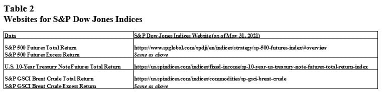
Table 1 provides the Bloomberg tickers for the Brent front-to-back spread; the table also displays the Bloomberg tickers for both the total return series and the excess return series for Brent futures contracts, U.S. 10-Year Treasury Notes futures contracts, and E-Mini S&P 500 futures contracts.  With one exception, each of these return series are described at their respective S&P Dow Jones Indices websites; Table 2 provides the links for five of the six return series.  

 

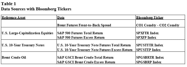
The sixth return series, the U.S. 10-Year Treasury Notes Futures Excess Return, is described in Citigroup Global Markets Holdings (2021).

 

Results

Table 3 provides the 2000-to-2020 yearly performance of (1) the neutral portfolio (60% equities and 40% Treasuries), (2) the static allocation across the three asset classes (30% equities, 30% oil, and 40% Treasuries), and (3) the conditionally determined strategy (the dynamic allocation portfolio).  Table 4 provides the summary statistics for the three portfolios.

Over the full dataset, the “dynamic allocation” portfolio’s compound annual growth rate (CAGR) was 10.0%, which outperformed the two static allocation portfolios’ returns.  The traditional portfolio earned 6.6% while the 30% equities/30% oil/40% Treasuries portfolio earned 6.7%.  The dynamic allocation portfolio’s Sharpe Ratio came in at 1.0 while the other two portfolios had Sharpe Ratios of 0.5.

Over the 2016-to-2020 timeframe, the dynamic allocation portfolio still outperformed the classic balanced portfolio with the former portfolio having a CAGR of 12.3% and the latter portfolio earning 10.8%.  The 30% equities/30% oil/40% Treasuries portfolio had the lowest returns of the three portfolios with a CAGR of 8.7%.  The dynamic portfolio’s Sharpe Ratio was 1.3 while the classic balanced portfolio’s Sharpe Ratio was 1.1.  The Sharpe Ratio of the 30% equities/30% oil/40% Treasuries portfolio was the lowest of the three portfolios at 0.7.

 

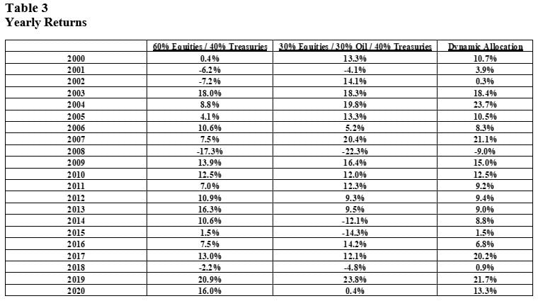
Note:  The Sharpe Ratios are calculated from the yearly data in Table 3.

 

Figure 1 shows the growth of $1 in each of the three asset allocations from January 2000 through December 2020. 

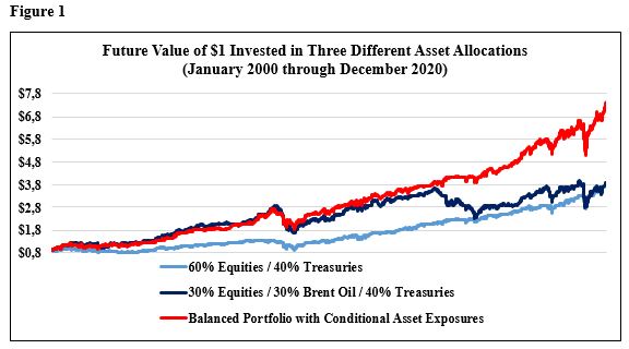
The performance of the classic balanced portfolio is represented by the blue line; the performance of the static allocation portfolio across the three assets is shown in the grey line; and the performance of the dynamic allocation strategy is displayed in the red line.

Source:  Premia Research LLC.

 

Impact of Publishing a Trading or Investment Strategy

The study’s results are highly suggestive of how to potentially improve upon a default allocation of 60% in equities and 40% in Treasuries, which is of heightened interest because of the renewed concerns of possibly entering into an inflationary era.  That said, one risk of publicly identifying investment or trading strategies that have historically had superior returns is that they will stop working as capital flows into them, a concern noted in Cochrane (1999).  But it may be that the particular dynamic asset allocation that is outlined in this article is sufficiently unusual as to prevent overcrowding in the strategy.

 

Impact of a New Paradigm in the Energy Markets on Portfolio Construction

Another concern with this paper’s results is its reliance on crude oil futures returns.  What will happen to such a strategy if crude oil no longer remains a crucial fuel in the global economy, given how, in the words of Neville et al. (2021), “electric vehicle technology [is] developing fast”?

Dale and Fattouh (2018) provide a framework for the prospect of “peak oil demand.”  Even if oil demand levels off, “[t]he world is likely to demand large quantities of oil for many decades to come.”  The key paradigm shift under a “peak oil demand” scenario is that there would be a break from “a past dominated by concerns about adequacy of supply.”  The world would be an entering an “age of [oil] abundance.” 

The utility of our dynamic allocation’s strategy signal is that it is a proxy measure of oil inventory scarcity.  And when there is a signal of surplus, the dynamic strategy does not include oil futures within its asset allocation.  Under a new paradigm of oil abundance, the strategy would be expected to default to the classic balanced portfolio of equities and Treasuries.  As a result, even with “peak oil demand,” an investor in the dynamic allocation strategy would plausibly be no worse off than solely investing in a classic balanced portfolio.  And then however long the current paradigm holds, the investor in the dynamic allocation strategy could potentially earn superior returns relative to a neutral portfolio of equities and Treasuries.

 

Conclusion

This article provided a brief (and therefore, not exhaustive) review of papers that are relevant to including commodities in traditional portfolios.  The topic has once again come to the fore over concerns on potentially entering into an era of inflationary surprises, which would not bode well for portfolios solely invested in stocks and bonds. 

Based on insights in prior research, this paper suggests a dynamic asset allocation into crude oil (and namely, into Brent futures contracts) when there is a (historically) reliable signal of scarcity.  Such a portfolio, which consists entirely of collateralized futures contracts, would have had a Sharpe Ratio of 1.0 from 2000-to-2020 and a Sharpe Ratio of 1.3 from 2016-to-2020.

A key concern with such a strategy is if the demand for crude oil is supplanted by alternative fuels.  Because the strategy is relying on the markets to provide a signal of oil scarcity or surplus, an investor can potentially be agnostic on when an energy transition could occur.  When a surplus in oil is signaled, the rules-based investment strategy defaults to a classic balanced portfolio.

As always, one must sound a cautionary note on the paper’s historical results since past performance is no guarantee of future results.  One hopes, though, that this article stimulates further interest in designing efficient hedges for the corrosive effect that inflationary surprises can have on traditional portfolios.

 

Endnote

The author gratefully acknowledges research assistance from Mark Shore, Chief Research Officer, Shore Capital Research and Adjunct Professor, DePaul University in Chicago.

 

References

Bouchouev, I. and L. Zuo, 2020, “Oil Risk Premia under Changing Regimes,” Global Commodities Applied Research Digest, Editorial Advisory Board Analysis, Vol. 5, No. 2, Winter, pp. 49-59. 

Citigroup Global Markets Holdings Inc., 2021, “Market-Linked Notes Based on the Citi Dynamic Asset Selector 5 Excess Return Index Due May 31, 2028,” Medium-Term Senior Notes, Series N, Pricing Supplement No. 2021-USNCH7499, Filed Pursuant to Rule 424(b)(2), Registration Statement Nos. 333-255302 and 333-255302-03, May 25.  Accessed via website: https://sec.report/Document/0000950103-21-008047/dp151852_424b2-us214250... on May 31, 2021.

Cochrane, J., 1999, “New Facts in Finance,” Economic Perspectives, Federal Reserve Board of Chicago, Third Quarter, pp. 36-58.

Dale, S. and B. Fattouh, 2018, “Peak Oil Demand and Long-Run Oil Prices,” Energy Insight: 25, Oxford Institute for Energy Studies, January.

Erb, C. and C. Harvey, 2006, “The Tactical and Strategic Value of Commodity Futures:  Unabridged Version,” Trust Company of the West and Duke University Working Paper, January 12.

Froot, K., 1995, “Hedging Portfolios with Real Assets,” Journal of Portfolio Management, Vol. 21, No. 4, Summer, pp. 60-77.

Gorton, G., Hayashi, F. and G. Rouwenhorst, 2013, “The Fundamentals of Commodity Futures Returns,” Review of Finance, European Finance Association, Vol. 17, No. 1, January, pp. 35-105. 

Levine, A., Ooi, Y. and M. Richardson, 2016, “Commodities for the Long Run,” National Bureau of Economic Research Working Paper No. 22793, November.

Neville, H., Draaisma, T., Funnell, B., Harvey, C. and O. van Hemert, Man Group Working Paper, 2021, “The Best Strategies for Inflationary Times,” May 25.  Available at SSRN:  https://ssrn.com/abstract=3813202 as of May 31, 2021.

Tchilinguirian, H., 2003, “Stocks and the Oil Market:  Low Stocks, Volatility, Price Levels, and Backwardation,” International Energy Agency – Oil Industry & Markets Division Presentation, Berlin, September 19.