Diversification and Insurance: Which Should Come First?

Modern portfolio theory suggests that the complex problem of investor welfare maximization subject to various constraints is best handled by jointly using three forms of risk management. First, diversification aims to harvest risk premia across and within asset classes with the lowest possible amount of risk and leads to the construction of well diversified performance-seeking portfolios (PSPs). Second, hedging aims to immunize a portfolio against certain risk factors and leads to hedging portfolios, including liability-hedging portfolios in asset-liability management, and goal-hedging portfolios in goal-based investing. It completes diversification in that it takes care of systematic risk factors, the exposures to which cannot be neutralized by diversifying a portfolio, while idiosyncratic risk is eliminated by diversification. Finally, insurance is captured via a dynamic allocation between a PSP and a hedging portfolio designed to secure an essential goal that can be the protection of a minimum amount of wealth or, more generally, the protection of a minimum amount of wealth relative to a benchmark. Fund separation theorems from dynamic portfolio theory (see e.g. the seminal paper by Merton (1973) and Martellini and Milhau (2012) for the incorporation of minimum funding requirements) show that the investment strategy that maximizes an investor’s welfare uses all three techniques.

This discussion raises the following question: if diversification and insurance (i.e., dynamic hedging) are not mutually exclusive techniques, is there an optimal order for them to be performed? Put differently, is it better to diversify a portfolio of insured payoffs or to insure a diversified portfolio? Since insurance has an opportunity cost, which takes the form of a limited participation in the upside of the PSP in favorable scenarios, compensating for the downside protection in unfavorable scenarios, and since diversification has no cost, intuition suggests that it should be more efficient to costlessly diversify away unrewarded risk before insuring the resulting portfolio at a cost. This lower opportunity cost is reflected in the lower price of the put option that protects against downside risk if the volatility of the underlying asset has been reduced first by diversification.

Several theoretical optimality results show that under certain assumptions, diversification should indeed come before insurance. El Karoui, Jeanblanc and Lacoste (2005) show that an investor who maximizes expected utility from future wealth with constant risk aversion and imposes a minimum wealth constraint should implement an extended form of option-based portfolio insurance (OBPI), where the underlying asset of the option is the portfolio that would be optimal in the absence of the constraint. The latter portfolio is diversified because the expected utility criterion favors returns but penalizes risk, but it involves the expected returns and covariances of constituents and the risk aversion parameter (Merton, 1973). When the objective is to maximize the probability of reaching a target wealth level while respecting a floor, Föllmer and Leukert (1999) and Deguest et al. (2015) establish that it is optimal to hold a knockout option that pays either the floor or the target, whose underlying asset is the “growth-optimal portfolio”, that is the portfolio that maximizes the expected logarithmic return.

These theorems are obtained in a stylized framework where continuous trading, leverage and short sales are allowed, all risk and return parameters are perfectly known and the criterion is expected utility or the success probability. In practice, it can be argued that since crashes and recoveries in risky assets are not perfectly synchronized, it might be worthwhile to have an asset-by-asset control of the amount of risk-free asset to be invested in – and this would be done by applying insurance first. In this context, this paper considers whether the question of which should come first, diversification or insurance, subsists in a context closer to real-world investment conditions than the theoretical environment in which the theoretical results are derived. We consider various diversification methods often used in practice, which avoid the estimation of expected returns and risk aversion. These are equal weighting, variance minimization, risk parity (Maillard, Roncalli and Teiletche, 2010) and maximum diversification (Choueifaty and Coignard, 2008). As far as insurance strategies are concerned, we test both constant proportion portfolio insurance (CPPI) and option-based portfolio insurance (OBPI), and we report several standard performance and risk metrics to compare the properties of the “diversification first” and “insurance first” approaches. A non-trivial methodological issue that arises in our study is how to construct a diversified portfolio of insured payoffs, given that the usual diversification methods require a covariance matrix estimate. We propose two estimators, both of which are consistent with the returns on the original securities, and one of which takes into account the composition of the insured portfolio.

Our results show that it matters whether insurance or diversification comes first. The big picture is that diversification before insurance tends to perform better than insurance before diversification in the long run, thereby confirming the aforementioned intuition about reducing the opportunity cost, but there are exceptions to this finding, since an equally weighted portfolio of CPPI-like payoffs outperforms a CPPI portfolio based on an equally weighted portfolio. Ultimately it seems that no one approach unambiguously prevails over the other, with respect to whether diversification or insurance should come first.

 

Diversification and Insurance Methods

We begin with a presentation of the tested diversification methods. Broadly speaking, they all implement the “don’t put all your eggs in one basket” principle, but they differ through their definition of the eggs and the baskets. In terms of financial theory, they all attempt to diversify away the idiosyncratic risk of constituents, which only increases portfolio risk without being rewarded, in order to maintain exposure only to systematic sources of risk, which are rewarded.

The simplest, sometimes coined “naïve”, interpretation of the principle is that a portfolio is best diversified when all dollars are evenly split across constituents, so that the portfolio is equally weighted. By construction, this strategy is immune to estimation risk because it does not rely on any parameter estimate, and this property makes it a difficult-to-beat benchmark for more sophisticated approaches that rely on mean-variance optimization (DeMiguel, Garlappi and Uppal, 2009b).

If information is available on the correlations and volatilities of the constituents, one can also diversify a portfolio by minimizing its expected variance, which leads to the global minimum variance (GMV) portfolio. An interesting practical property of this strategy is that it is not exposed to the estimation errors that plague expected returns, but it still requires a covariance matrix estimator, which is a non-trivial task when the constituents are non-linear payoffs like those of insurance strategies. It is also well known that GMV portfolios tend to be concentrated in a few securities, like low beta stocks (Green and Holliefield, 1992). As noted by Black and Litterman (1992), the observation that such portfolios lack diversification in the naïve sense can be an obstacle to their adoption by asset managers. The concentration issue can be addressed by imposing a minimum weight in each asset, or by constraining the sum of squared weights to a maximum, as proposed by DeMiguel et al. (2009a). A different idea to reduce concentration is to smooth the respective contributions of the constituents to portfolio volatility. Maillard, Roncalli and Teiletche (2010) thus introduce “risk parity” portfolios, in which all constituents have the same contribution to risk.

The fourth diversification method that we test is Choueifaty and Coignard’s (2008) maximum diversification. This maximizes the “diversification ratio”, defined as the weighted sum of constituents’ volatilities divided by the portfolio volatility. It can be shown that this ratio takes on its minimum value when all securities are perfectly correlated with each other, that is when there are no diversification opportunities. In contrast, the “maximum diversification portfolio” attempts to make the most of the diversification opportunities offered by imperfectly correlated constituents.

While reducing – and ideally removing – idiosyncratic risk, diversification methods do not eliminate the risk of large short-term losses, mostly due to systematic risk factors, as can be seen from the top panel in Table 1, which displays statistics on the performance of portfolios of large US stocks. All portfolios but the minimum variance one lost more than 20% within at least one year and the loss was as high as 30.2% for the equally weighted portfolio.

To avoid such large losses, one must employ another risk management technique, which is insurance. In this paper, we consider two popular strategies, namely CPPI and OBPI. Both have a non-linear payoff in the value of their underlying risky asset, and this payoff is in fact convex owing to the elimination of values that fall below the floor. In CPPI, insurance is achieved via a dynamic allocation to the PSP and the floor-replicating portfolio (FRP), which is a pure discount bond with a face value equal to the targeted minimum amount of wealth. At each rebalancing time, the PSP weight equals the risk budget, calculated as the distance between current wealth and the floor, times a multiplier m. The strategy is exposed to gap risk, which is the risk of breaching the floor if the PSP underperforms the FRP by a large amount between two rebalancing dates.

OBPI is another form of insurance, which uses the replication of put options written on the PSP to insure a portfolio against the risk of losses in the PSP value. The payoff is then equal to the maximum between the floor wealth level, say M, and some multiple of the PSP value. If S and W denote the respective payoffs of the PSP and the insured portfolios, then W has the form:

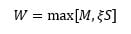
where is some number less than 100%, which represents the fraction of the performance of the PSP that is captured when the protective put is out of the money. The insured payoff can be rewritten to highlight the put payoff:

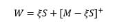
The work of Black and Scholes (1973) shows that the put option is equivalent to a dynamic trading strategy involving the PSP and a risk-free asset.

 

Monte-Carlo Analysis

To make comparisons between the “diversification first” and “insurance first” approaches, we need a set of risky assets, which will serve as the constituents of the “diversified first” portfolios and as the underlying assets of the “insured first” portfolios. We begin with a set of assets whose returns are generated from a stochastic model in order to abstract away from parameter estimation issues. Each security price follows a Geometric Brownian motion, meaning that returns are independent and identically distributed over time. To fix the correlations and the volatilities of these securities, we calculate the sample covariance matrix of the weekly returns on 496 large US stocks from December 2016 to December 2018 and we apply the eigenvalue clipping procedure of Laloux et al. (2000) to separate statistical noise from informative signal in returns. The 496 expected returns are sampled from a log-normal distribution, which ensures that they are positive, with a mean of 0.073 and a standard deviation of 0.049. These values are borrowed from Martellini, Milhau and Tarelli (2014), who study the distribution of expected returns estimated by the three-factor Fama-French model.

Based on these parameters, we simulate 10,000 scenarios for asset prices, and we apply the diversification and insurance methods. The horizon of simulations is one year, and the insurance strategy applied to the diversified portfolios or the individual assets aims to avoid losses greater than 20% over this period. In this stylized setting, it is possible to simulate the values of a continuously rebalanced CPPI portfolio, which eliminates the gap risk that arises with discrete rebalancing.

An interesting property of the Geometric Brownian motion assumption is that it allows for analytical calculation of the covariances between the non-linear payoffs of insurance strategies. Detailed expressions are given in the Appendix and can be used to calculate the weights of diversified portfolios invested in the insured constituents.

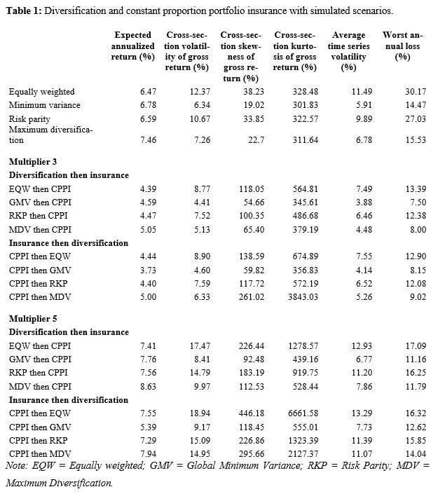
Table 1 shows that with the minimum variance, risk parity and maximum diversification schemes, performing diversification before insurance results in a greater average return, especially with a multiplier of 5. The biggest return spread is achieved with the GMV portfolio and a multiplier of 5, since the diversification first approach earns 7.76% per year, versus 5.39% for the GMV portfolio of insured constituents. On the other hand, insurance first leads to more volatile portfolios, whether volatility is measured as the standard deviation of the gross return, or as the average time series volatility of weekly returns across scenarios. (Time series volatility is calculated for each simulated scenario, and the 10,000 values are then averaged, while the cross-section volatility of the gross return is the standard deviation of the one-year return across scenarios.) The comparison in terms of higher-order moments also yields mixed results: with insurance first, skewness is greater, which is a positive feature of the distribution, but kurtosis is greater too, which is undesirable.

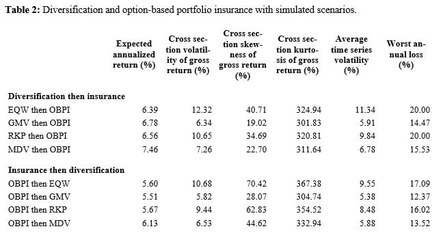
If insurance is done with OBPI, like in Table 2, the domination of diversification first in terms of average returns appears more clearly since it occurs for all four diversification methods, including equal weighting. On the risk side, it is insurance first that delivers lower volatilities, in contrast with CPPI, but it also has higher kurtosis, like for CPPI.

Empirical Analysis

We now make a comparison of the two approaches in the context of an empirical analysis based on actual stock returns.

 

Methodology

The investment universe is built by taking a snapshot of the 500 largest stocks existing in the CRSP database at each quarterly date from November 1984 to December 2018. It shows close correspondence to the S&P 500 universe. In order to ensure relevance of the results to large investors, the eligible universe to be used in testing is then filtered from the raw universe on a liquidity measure which is informed by turnover (average daily value traded) and the proportion of zero-trade days, both measures being obtained from FactSet’s Standard Datafeed database. The raw daily turnover is smoothed using a moving median with a lookback window of one year. The daily smoothed turnover for each stock is then ranked in the cross-section from highest to lowest, and the stocks with the highest values at each rebalance date are selected. A zero-trade day filter is then applied at each rebalance time in order to filter out stocks that have not traded for more than 15% of the trading days over the lookback window of two years. These are excluded from the eligible universe at each rebalance.

The minimum performance constraint applied to insured portfolios is now reset periodically: the objective is not to lose more than 20% between two consecutive reset dates. The reset frequency is aligned with the rebalancing frequency of diversified portfolios, which we take to be 60 trading days. This is a practical requirement for the insurance first study, since a reset must take place whenever the list of constituents changes. The choice of the floor-replicating portfolio is dictated by the performance constraint: it is a pure discount bond that matures on the next reset date. Insured portfolios are rebalanced every day to eliminate gap risk with a high confidence level. For the OBPI method, we do not assume that the protective put readily exists, and we instead implement its dynamic replication strategy, which is based on Black and Scholes’ (1973) dynamic option replication method.

A 500-day data window of returns is used whenever parameters need to be estimated: these parameters are either the covariance matrix of constituents, for diversified portfolios, or the volatility parameter required by the dynamic option replication strategy.

 

Covariance Matrix of Insured Portfolios

Unlike in the Monte-Carlo analysis, the data-generating process for stock returns is not known, so the covariances between non-linear payoffs cannot be expressed in terms of the risk and return parameters of the underlying assets. The first idea is to estimate them as the covariances between the returns on the insured portfolios, which themselves are calculated from the covariances of the constituents and the weights. In detail, the covariance between the returns of two insured portfolios, r1 and r2, is

 

where is the weight of the risky asset in portfolio i,  is the covariance between the two risky assets,  and  are the covariances between the risky assets and the bond, and  is the bond variance. Weights are rule-based and observable, and covariances of constituents are estimated from data over the past two years. We refer to this estimator as the time-consistent estimator.

A potential problem with this method, however, is that it can lead to highly concentrated portfolios after a stock has experienced a severe loss. Indeed, the insured portfolio built on that stock is then largely dominated by the bond, and the bond has low variance compared to the stock and low covariances with the other stocks. As a result, a GMV or risk parity portfolio of insured stocks is dominated by one constituent only. For this reason, we also test an alternative estimator, which is simply the covariance matrix of the underlying risky constituents.

 

Effect of Insurance on Individual Constituents

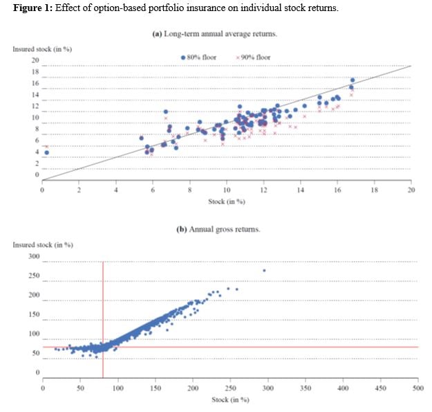
Figure 1 shows the annual returns averaged over the period 1970–2018 in Panel (a) and the annual returns in Panel (b). In Panel (a), the opportunity cost of insurance clearly appears, since most dots are located below the diagonal line: in other words, most insured portfolios have lower long-term returns than their underlying stocks, especially if the minimum annual gross return is raised from 80% (the base case) to 90%. On the other hand, Panel (b) shows the expected truncation of annual gross returns less than 80%, up to the violations caused by imperfect option replication.

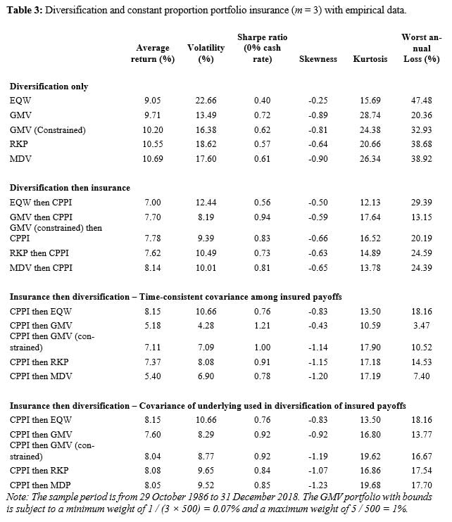
The empirical results confirm that the order of diversification and insurance does have an impact, but the choice of the covariance matrix estimator appears to have an impact too. With CPPI as the insurance method (in Table 3) and the time-consistent estimator, the diversification first approach delivers higher long-term returns for all diversification methods, except for equal weighting. It also leads to more volatile portfolios, but the net impact on the Sharpe ratio is either positive or negative depending on the diversification method. For instance, the GMV portfolio of insured stocks has a volatility of 4.28% and earns 5.18% per year, while the CPPI portfolio that has the GMV portfolio of stocks as its underlying asset posts a volatility of 8.19% but a better return of 7.70%. The ranking of the two approaches in terms of skewness or kurtosis also depends on the diversification method.

The use of the covariance matrix of underlying assets raises both the average returns and the volatilities of strategies implementing insurance first, but it also yields more negative skewness and increased kurtosis. With this estimator, insurance first yields higher returns than diversification first for 3 out of 5 diversification schemes and higher Sharpe ratios for 4 of these schemes.

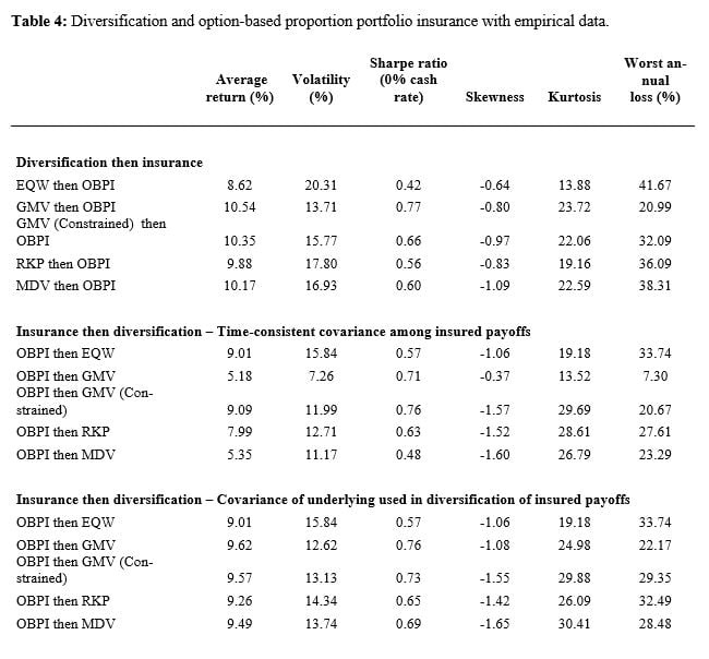
With OBPI in Table 4, the “insured first” portfolios built from the covariance matrix of stocks also display higher returns and volatilities than those based on the time-consistent matrix. Nevertheless, they are dominated in terms of performance by the “diversified first” portfolios, except when diversification is performed by weighting constituents equally. In all cases, diversification first also produces less negative skewness.

Conclusion

The order in which diversification and insurance are performed matters, but the optimal order appears to depend on the diversification and the insurance methods and on how the covariance matrix of insured payoffs is estimated. The results from the above numerical and empirical analysis indicate that with OBPI as the insurance technique, there is a clearer domination of diversification first in terms of long-term returns although insurance first delivers lower volatilities. This can be taken as a loose confirmation of the theoretical optimality (in the sense of expected utility maximization) of OBPI written on a diversified portfolio. With CPPI, the results are more mixed, and insurance first produces higher returns if it is combined with equal weighting. In all cases, using the covariance matrix of the underlying assets to diversify across insured assets leads to higher returns than estimating covariances across insured assets by taking into account the composition of each insured portfolio.

Overall, we find that for a given insurance payoff (CPPI or OBPI), the choice of the diversification scheme matters in the sense that equal weighting, variance minimization, risk parity and maximum diversification lead to different outcomes. Conversely, for a given diversification scheme (equal weighting, variance minimization, risk parity and maximum diversification), the choice of the non-linear insurance payoff matters in the sense that CPPI and OBPI lead to different outcomes. While diversification and insurance are most often performed independently from each other, our findings suggest that a closer analysis of the interaction between these fundamental risk management techniques may lead to welfare improvements for investors.

 

Appendix: Covariances Between Non-Linear Payoffs

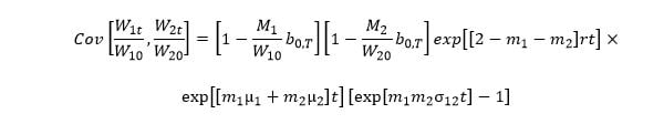
Consider two insured portfolios with respective minimum wealth levels M1 and M2 and initial investments W10 and W20, and assume that the prices of the two underlying risky assets follow Geometric Brownian motions with expected returns m1 and m2, volatilities and and covariance . Let r denote the short-term interest rate. 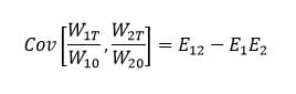If the portfolios are insured by the CPPI method with respective multipliers and , then the covariance between their values at time t is:

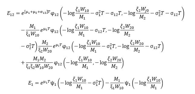
Now suppose that both portfolios are insured by OBPI. The formula for their covariances is more complex and involves the coefficients of access to upside, and . We obtain:

where

is the cumulative distribution function of a normal distribution with mean and variance  , and  is the joint cumulative distribution function of two normal distributions with means and , variances   and , and covariance  and have similar definitions.

 

The research from which this article was drawn was produced as part of the EDHEC-Risk Institute/FirstRand research chair on “Designing and Implementing Welfare-Improving Investment Solutions for Institutions and Individuals”.

 

 

References

Black, F. and M. Scholes. 1973. The Pricing of Options and Corporate Liabilities. Journal of Political Economy 81(3), 637-654.

Black, F. and R. Litterman. 1992. Global Portfolio Optimization. Financial Analysts Journal 48(5), 28-43.

Choueifaty, Y. and Y. Coignard. 2008. Toward Maximum Diversification. Journal of Portfolio Management 35(1), 40-51.

DeMiguel, V., L. Garlappi, F.J. Nogales and R. Uppal. 2009a. A Generalized Approach to Portfolio Optimization: Improving Performance by Constraining Portfolio Norms. Management Science 55(5), 798-812.

DeMiguel, V., L. Garlappi, F.J. Nogales and R. Uppal. 2009b. Optimal Versus Naive Diversification: How Inefficient is the 1/N Portfolio Strategy? Review of Financial Studies 22(5), 1915-1953.

El Karoui, N., M. Jeanblanc and V. Lacoste. 2005. Optimal Portfolio Management with American Capital Guarantee. Journal of Economic Dynamics and Control 29(3), 449-468.

Föllmer, H. and P. Leukert. 1999. Quantile Hedging. Finance and Stochastics 3(3), 251-273.

Green, R. and B. Hollifield. 1992. When Will Mean-Variance Efficient Portfolios Be Well Diversified? Journal of Finance 47(5), 1785-1809.

Laloux, L. P. Cizeau, M. Potters and J.P.  and Bouchaud. 2000. Random Matrix Theory and Financial Correlations. International Journal of Theoretical and Applied Finance 3(3), 391-397.

Maillard, S., T. Roncalli and J. Teiletche. 2010. The Properties of Equally Weighted Risk Contribution Portfolios. Journal of Portfolio Management 36(4), 60-70.

Martellini, L., V. Milhau and A. Tarelli. 2014. Estimation Risk versus Optimality Risk: An Ex-Ante Efficiency Analysis of Alternative Equity Portfolio Diversification Strategies. Bankers, Markets and Investors 132, 26-42.

Martellini, L. and V. Milhau. 2021. Diversification and Insurance: Which Should Come First? EDHEC-Risk Institute Publication.

Merton, R.C. 1973. An Intertemporal Capital Asset Pricing Model. Econometrica 41(5), 867-887.

Martellini, L. and V. Milhau. 2012. Dynamic Allocation Decisions in the Presence of Funding Ratio Constraints. Journal of Pension Economics and Finance 11(4), 549-580.