How Can Strategic Investors Deal with Climate Uncertainty?

• Climate scenarios are indispensable to investors because of the unprecedented nature of climate change. Since market ‘expert knowledge’ is not available, they must come equipped with probabilities.
• Current scenarios were created with policy goals in mind. Despite their excellent quality, they do not serve the needs of investors well. In particular, they have no probabilities associated with them, and do not adequately convey the huge uncertainty in climate outcomes.
• We show how it is possible to create probability distributions of climate outcomes, that allow investors to appreciate the degree of uncertainty they face, and to judge which realizations are more likely, and should therefore command greater attention.

 

 

1 - The Climate Challenge for Strategic Investors

Climate risk is a new source of concern for strategic investors. There are many reasons why they should be worried. First of all, like market risk, it is a systematic risk, and, as such, cannot be eliminated by diversification. Second, exactly because it is systematic, it may in principle attract a risk premium: whether this should be positive or negative (or, zero) is, however, far from easy to ascertain.[1] Third, climate risk is by its very nature radically new, and investors cannot refer to an accepted ‘playbook’ of responses, as they would in the case of, say, market or credit risk – they are stepping into uncharted investment territory.

In order to tackle these sources of concern, investors must be able to form an idea of the most plausible climate outcomes; of what may ‘lurk in tails’; and of ‘thickness’ of the distribution between the central moment and the tails of the distribution – roughly, speaking, of the degree of uncertainty. This explains why they have recently looked with renewed interest at climate scenario analysis and climate stress testing. We shall argue that this interest is well placed, but also that, in the climate risk domain, these analytical tools must be embedded in a probabilistic framework.

One often hears the objections that market scenarios are routinely used by practitioners without explicit probabilities attached to them. Why should climate scenarios be different? The reason is that, when it comes to market scenarios, investment professionals have (often painfully) built a precious body of expert knowledge based on a hundred-years-plus of financial data. This body of knowledge allows them to carry out ‘informal’ probability assessments of the likelihood of a market scenario – in practical terms, it allows them to tell them whether and how much they should worry about the scenario in question. And, if one really wanted, a more formal probabilistic assessment of the likelihood of a market scenario could always be carried out based on the historical frequency of past market moves. Not so, however, in the case of climate outcomes, whose dynamic and unprecedented nature brings to the fore completely new challenges.

Unfortunately, the best-known and most-widely-used climate scenarios (which have been created under the auspices of the Intergovernmental Panel on Climate Change) do not have any probabilistic dimension at all, and this is one of the reasons why they do not serve the needs of investors well. This is not because the existing scenarios are of poor quality – far from it: they are of excellent quality, and teams of world-known experts have contributed to their formulation. However, these scenarios were not created with the need of investors in mind because they were built with a policy focus.

Shouldn’t policy-useful scenarios also serve the needs of investors well? Not necessarily. First of all, in the policy area, it is reasonable to err on the side of caution (a `policy tilt’ underpinned by the so-called ‘precautionary principle’). When it comes to investing, however, there is no ‘safe way to be wrong’: for a long-term investor faced with climate risk, the consequences of an excessively prudent asset allocation can be every bit as severe as the results of an overly aggressive stance.

Second, as mentioned, the currently used IPCC-endorsed scenarios have completely eschewed any assessment of their relative likelihood. Because of their policy origin, this makes historical sense, but it is of no use to financial planners, who need an understanding of what the most plausible outcomes may be; of how uncertain we are about these estimates; and of what may happen if things go ‘really wrong’ – in short, what they need is a probability distribution of climate outcomes.

 

2 - From Scenarios to Probability Distributions

For these reasons, we have already argued (Rebonato, Kainth and Melin, 2024) that the probability agnosticism of the IPCC scenarios makes them poorly suited to the needs of investors. Most contentiously, we intend to show here that the very language of scenarios is poorly suited to dealing with climate uncertainty, and that investors must familiarize themselves with the related but distinct dialect of probability distributions. (The required step is not as big as it might seem: after all, investors routinely handle the concepts of expected returns and variance – and, when they do so, they often have in the back of their minds an underlying normal distribution with these parameters. The challenge is that, when it comes to climate outcomes, their distribution is going to be far more skewed and even more fat-tailed than the distribution of market outcomes.)

To understand why the language of scenarios is poorly suited to the climate domain, it pays to look in some detail at the IPCC-endorsed scenarios, which have become, or have inspired, the current benchmark scenario approach.[2] These are made up of a combination of socioeconomic narratives (SSPs), and of representative pathways of carbon emissions (RCPs). The socioeconomic narratives cover such diverse aspects as demographic growth, technological progress, and economic development – to say nothing of political and social features such as ‘resurgent nationalism’ or ‘growth of inequality’. These narratives are compelling and, the more detailed they are, the more convincing they sound. The problem is that, with so many variables at play, there is a staggering number of possible ways to combine them. Since each combination is a possible narrative, there are far too many ‘possible words’ for the human mind to handle with any ease: if we allow for as few as three variables, each allowing a ‘high’, ’medium’ and ‘low’ state, 162 scenarios result. And this is why the IPCC has created only six such narratives. Each one is both engaging and coherently structured. However, these six possible ways in which the world may evolve over the rest of the century certainly do not span the full range of possible outcomes; and, since they have not been associated with any probability, one cannot even argue that these are the most representative or likely narratives – the ones that should command the investors’ undivided attention. They are just six ‘plausible’ stories.

This matters. When one works out what, say, climate damages may be if the third narrative unfolded, one is in effect conditioning on the very specific realization of all the socioeconomic variables in that narrative: which means that the calculated damages only apply if that particular narrative unfolds – an event about whose probability investors are given no indication. It comes to little surprise, then, that the Network for the Greening of the Financial System should have chosen the narrative with the monicker ‘Middle of the Road’ as the only narrative around which all their scenarios have been built. Given the name, it is understandable that it should have been interpreted as the most likely, and therefore singled out as the one worthy of most attention: but the name hides the fact that no such probabilistic statement is made in the SSP/RCP approach!

Since, in isolation, each narrative is plausible, an investor may well form her own opinion about its likelihood; however, she will immediately note that many possible combinations of the underlying variables are missing (for instance, the plausible ‘Green Growth’ scenario of high abatement obtained alongside high economic growth and declining population growth is not present). In technical terms, the six IPCC-chosen scenarios do not span the sample space, and therefore one cannot just associate them with probabilities adding up to 1.

The situation is even more complex. The multitude of pathways that lead to a given climate outcome still do not uniquely define what an investor is truly interested in, ie, the climate damages that may affect their portfolio: to link temperatures to damages one needs a damage function – and, as discussed in Rebonato, Kainth and Melin (2024) and Kainth (2023), this introduces additional uncertainty. And the temperature at the end of the century (or on any other date) will also depend on the abatement policies chosen along the path. Even if, again, we only allow these two variables (the severity of damages and the aggressiveness of the abatement policy) to assume a ‘low’, a ‘medium’ or a ‘high’ value, this still brings about a further multiplication of scenarios. Once we allow also for the damage exponent to assume a ‘low’, ’medium’ or ’high’ value,[3] the 162 scenarios mentioned above become 4,374. So, the damages associated with an investor’s portfolio are conditional on a certain realization of the demographics, of the economy, of the technology, of the abatement aggressiveness and of the damage exponent – and, even if we rely on bold assumptions, we have thousands of such combinations. Admittedly, some combinations may be highly unlikely, but the plausible combinations are far more than six! It is clear that, in the climate-risk context, a naïve scenario approach is fraught with huge problems. This way of presenting the problem, however, also points to its possible resolution.

Suppose for a moment that the scenario builder has chosen the low, medium or high values for each of the state variables to have the same probability. If this is the case, we can group the thousands of (now equiprobable) scenarios into subsets that produce approximately the same damages, and associate to these damages a probability. For instance, one may find that, out the 4,374 overall scenarios, 87 produce portfolio damages between X and Y percent: this means that probability of portfolio losses in that range is approximately 87/4,374 = 2%. The way we have presented the ‘problem with scenarios’ has naturally led to probability distributions, and these, we claim, are the correct tools for a problem as complex as climate risk.

The procedure we have sketched was of course predicated on the modeller’s ability to choose ‘low’, ‘medium’ and ‘high’ values of equal probability.[4] This is clearly a challenge. For some variables, such as GDP growth, we may have a wealth of historical data spanning centuries that can be extrapolated into the future. For technological progress, we may also have empirical data about the pace of innovation observed in the recent past, and some grounds for projecting future levels of technological development and their dispersion. But quantities such as the ‘aggressiveness’ of an abatement policy pose a much greater challenge. Even in this case, however, something meaningful can be said.

 

3- Looking Under the Bonnet – What the SSP/RCP Scenarios Imply

To understand both how difficult it is to assign probabilities to quantities such as policy aggressiveness, and how one may try to solve the problem, let us go back to the SSP/RCP scenario framework. We have so far looked mainly at the narrative but, as mentioned, these are coupled to different degrees of abatement aggressiveness via the Representative-Carbon-Pathway variable – a quantity that can be intuitively understood as the temperature resulting from that policy.[5] The way the coupling is achieved is by tuning the degrees of freedom of the IPCC-approved models to reflect the chosen narrative. These fine-tuned (‘calibrated’) models then optimize a single variable, the carbon tax, in such a way as to obtain the desired horizon temperature with the minimum cost: the carbon tax is assumed to be spent in the most efficient way on the abatement and removal technologies necessary to limit the temperature increase to the desired value.

This seems a reasonable enough procedure. However, the users of the IPCC-endorsed probability-agnostic scenarios have no way of knowing (short of looking carefully looking under the bonnet of the SSP/RCP engine as we have done) whether the ‘solution’ (the carbon tax) found by the model makes economic sense. Very few users, for instance, are aware that a 2 C warming is just not possible for the Regional-Rivalry SSP3 – which means that it has zero probability. If we recall that, globally, we spend between 3% on education and defense, and about 8% on the biggest spend item of all, healthcare, surely these levels of taxation must be associated with very low probabilities – probabilities that are inherited by the associated SSP/RCP combinations, ie, scenarios. However, all the scenarios are presented on the same probabilistic footing.

One can also look at the problem from a technological, rather than fiscal, angle. Let us consider the combination of the Middle-of-the-Road narrative with the goal of keeping the temperature increase under 1.5°C. Under this combined scenario, in ten years' time (from 2020 to 2030) abatement expenditures would climb from 8% to almost 60% of GDP. Even assuming no real GDP growth, this would equate to approximately $60 trillion devoted in 2030 to the installation of wind turbines and solar panels. Let us neglect for a moment the fiscal plausibility of such a level of taxation. We can still perform some quick back-of-the-envelope calculations to get a feel for the technological feasibility of this scenario. To keep the argument as simple as possible, let us neglect direct air capture and carbon sequestration and storage (which are in any case likely to play a minor role between now and 2030), and let us assume that the burden of decarbonization of the whole economy (not just of the energy sector) is split 50-50 between solar installations and wind turbines.

Assuming a cost of $2-4 million dollars for a wind turbine, this equates to 10 million turbines being installed every single year (and the pace of turbine instalment to be increased in the following decades). But, according to the Global Wind Energy Council, the total installation of wind turbines in the world to date (cumulative, not per annum!) has been 341,000. Clearly, also simple technological considerations indicate that the probability of this scenario combination should be extremely low. But since the investor using the scenarios are nowhere told of the low likelihood of these ones, they are given no indication about where they should ‘look for climate trouble’. As explained in Section 2, what investors require is a probability distribution of possible climate outcomes, but this is not part of the current scenario landscape. We therefore move to showing how it can be obtained.

 

4 - Building Probability Distributions for Climate Outcomes

When it comes to probability distributions of climate outcomes, one must distinguish between baseline and policy distributions: the former apply to a world in which no abatement actions are taken; the latter consider the effect of abatement policies of different aggressiveness. Creating the policy distribution is clearly more challenging, as one must also take into account the effect on temperatures of different courses of climate action, which are highly uncertain. Policy distributions can therefore be either conditional, when one abatement path is assumed to prevail; or unconditional, when one averages over all the possible abatement policies, each weighted by its probability of occurrence. We shall see how this can be done.

For both types of distributions, a good starting point is the Kaya (1990) identity, which, for each region, expresses emissions as the product of the Population, times how rich the region is (GDP/Population), times how much energy this region requires to produce one unit of GDP (Energy/GDP), times the amount of emissions required, given the technology of that region, to obtain one unit of energy (Emissions/Energy):

Emissions = Population x GDP/Population x Energy/GDP x Emissions/Energy  (1)

The blueprint for arriving at a distribution of climate outcomes from this relationship then unfolds as described below, for the baseline case first (Section 4.1) and for the policy case next (Section 4.2).[6]

 

4.1 – The Baseline Case

Let’s consider the simpler baseline case first – the case, that is, of no policy action. Empirically, one finds that both the energy intensity of GDP and the emission intensity are a (noisy) function of GDP/person.[7] The rate of growth of the population is also found to display a statistically significant dependence on GDP/person. Therefore, all the terms on the right-hand side of Equation (1) can be expressed as some function of GDP/person, plus residual noise. As an illustration, Figure 1 shows the (noisy but clear) relationship between the rate of growth of the population and GDP/person (in thousands of $, on the x axis). One can obtain these relationships directly from empirical data, or one can reverse-engineer them from the output of the SSP/RCP models, as described in Rebonato, Kainth and Melin (2023).[8]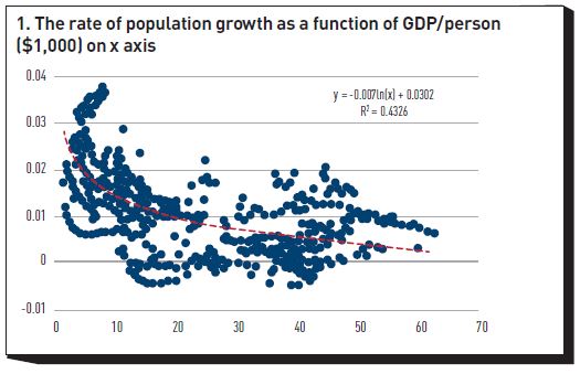

In either case, the key point is that there exist a number of well-established economic models that can produce distributions of GDP (and, as a by-product, of GDP/person) at various horizons. Thanks to the noisy relationships between energy intensity, population growth and emission intensity on the one hand, and GDP/person on the other from a distribution of GDP/person via the Kaya identity, one can therefore obtain a distribution of emissions. From this, well-established climate models can produce a distribution of temperatures. When these are coupled with a chosen damage function, these temperature distributions can then be related to distributions of economic damages (ultimately, impairments to cashflows).

Each of these steps requires, of course, careful handling and adds significant uncertainty, but the conceptual path to arrive at a distribution of climate outcomes in the baseline case is clear enough. One `simply’ has to map a distribution of future economic output (something that can be directly obtained as a by-product from any of the many Dynamic Stochastic General Equilibrium models in the literature) onto a distribution of future climate damages. The numerical challenges are non-indifferent, but the conceptual path is well-trodden. To deal with the policy case, one must be more creative.

 

4.2 – The Policy Case

The challenge ahead of us is how to create a distribution of climate outcomes in the presence of abatement policies. If the scenario user wanted to explore how a chosen abatement policy would change the baseline distribution, the only modification required would be to alter the term Emissions/GDP in the Kaya identity to reflect the effects of the chosen policy. All the plumbing already in existence to handle the baseline case would remain unchanged. This is simple enough, but of limited use.

What an investor would really like to have access to is not a distribution of damages dependent on a particular abatement path prevailing, but a damage distribution that reflects the unavoidable uncertainty about courses of abatement policy. This can be arrived at as follows.

First of all, as we explain in Rebonato, Kainth and Melin (2024), one can establish a close mapping between the optimal carbon tax and the aggressiveness of an abatement policy. The details are somewhat subtle, but the intuition is clear: since all the carbon tax is assumed to be spent on (efficient) abatement, knowing one quantity is almost tantamount to obtaining the other. And, once the abatement path corresponding to a certain carbon tax is given, well-established climate-physics equations can translate this abatement into a temperature distribution. As we have seen, this is then the input to the damage function. So, in the policy case the huge complexity of the problem can be, effectively if not perfectly, reduced to a much simpler problem: determining the distribution of either the average aggressiveness of the abatement policy, or of today’s carbon tax.[9] This then raises the question: Can we say something about the likelihood of different levels of carbon taxation?

To some extent, we can. One may want to take an extremely non-committal approach, in which as little as possible is assumed about our state of knowledge of future abatement policies. Even in this case, fiscal, the monetary and technological ‘soft constraints’ can tell us something informative about the distribution of possible carbon tax levels. More precisely, one can still use the fiscal and technology considerations discussed in Section 3 to limit the possible/plausible tax levels to a finite (and not-too-wide) range. In this non-committal approach (if, that is, one really believed that nothing more can be said than which values for the social cost of carbon are possible and impossible), one can then assign equal probability to each level of the carbon tax within the range. It is difficult to believe, however, that such a diffuse prior is the best description of our level of knowledge about what the possible carbon tax could be. There are several possible approaches to enrich our information set, and we briefly discuss one such possible avenue.[10]

There have been extensive surveys of what economists think the ‘correct’ carbon tax should be (Tol, 2023), with the polled estimates spanning a very wide range. The key observation is that this disparity of opinions generates in itself a distribution of carbon tax levels – and since, as we have seen, this quantity is very closely linked to the level of abatement, one can directly obtain a distribution for ‘abatement aggressiveness’. Admittedly, what one can obtain following this procedure is the distribution of opinions of economists (who, among other things, do not have to face re-election). For this and other reasons, the distribution of economists’ views therefore need not coincide with the distribution of politicians. One can, however, observe differences between economist-generated estimates of the carbon tax produced in the past, and the size of the contemporaneously enacted subsidies and taxes put in place by politicians. This observed variance can then be used to shift the distribution of carbon taxes recommended by economists so as to make it more representative of what politicians would actually do.

This transformation, while conceptually simple, is far from trivial, and it is a current topic of active research at EDHEC-Risk Climate Impact Institute. The overall underlying idea, however, is very intuitive: to move from the baseline case to the policy case, probability distributions must also take into account uncertainty about the abatement aggressiveness. As mentioned, this is closely related to the level of carbon taxation. About this we can estimate, first, what is possible; second, how this uniform distribution should be altered to account both for best expert opinion (the economists’ views) and for the inevitable wedge between what is considered theoretically optimal and what has been implemented. The engine to evolve in a consistent manner all the terms of the Kaya identity is then provided by an integrated assessment model (specifically, a much-extended and scenario-repurposed version of the Dynamic Integrated Climate-Economy model (Nordhaus and Sztorc (2013)).

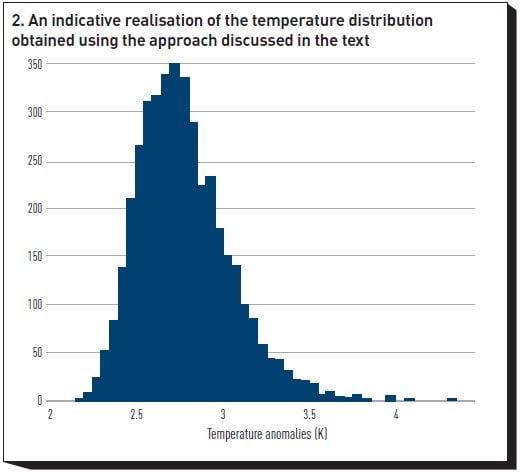
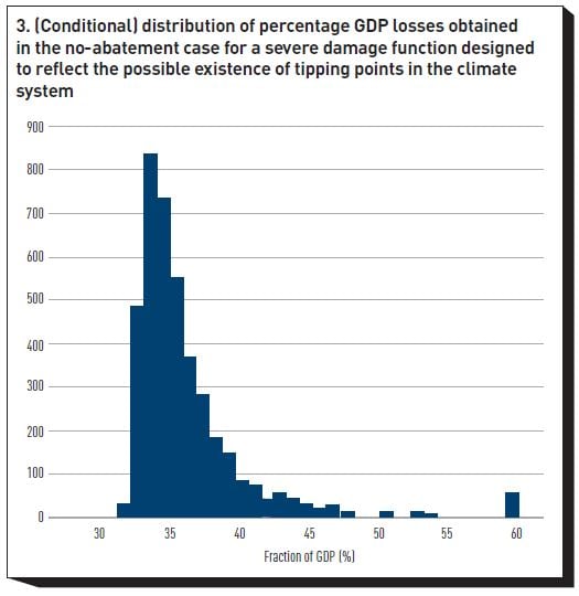
Figure 2 shows an indicative graph of the temperature distribution obtained using this approach, and Figure 3 displays a distribution of the possible damages corresponding to a no-action policy, expressed as percentage losses of 2100 GDP. (We stress that these GDP losses were obtained with a particularly severe damage function, which allows for the presence of tipping points in the climate system. They do not necessarily represent our best estimate of damages for the assumed policy course and are only presented to show that a DICE-like engine can produce substantial losses to economic output. Whether the damage function used to obtain Figure 2 is the most appropriate one is an empirical question, about which we are carrying out innovative research.)

 

 

 

5 – Conclusions: What Can Investors Do With This Information?

In this note we have advocated the use of probability distributions, rather than discrete scenarios, to investigate the effects of climate risk on an investor’s portfolio-allocation decisions. The procedure has been painted with a very broad brush, and the reader is referred to our technical publications for finer details, but the general idea should be sufficiently clear. What remains to be discussed is how investors can use this information is practice – also in this case, space constraints only allow us to do so from a 30,000-foot perspective.

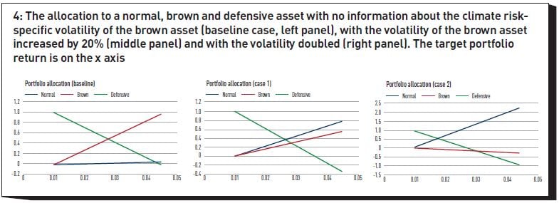
The first observation is that information about just the dispersion of outcomes can significantly change the portfolio allocation. To illustrate the point, Figure 4 shows an extremely simple allocation problem, where the portfolio manager had to decide how to split their wealth between a defensive, a ‘green’ and a ‘brown’ asset. The exercise is carried out first with no information about the climate-risk specific volatility of the brown asset (baseline case, left panel); next, with the volatility of the brown asset increased by 20% (middle panel); and finally with the volatility doubled (right panel). The target portfolio return is on the x axis. In all the cases considered, the expected returns from the different assets were not changed. Note how the allocation to the brown asset changes dramatically, from being the dominant asset in the left panel, to being shorted in the rightmost panel – purely as a function of the uncertainty in its returns. The intuition is clear: even if the expected returns do not change, increasing the climate sensitivity increases the volatility, and decreases the Sharpe ratio. (For a fuller discussion, see Rebonato, Kainth and Melin (2023)).

 

This stylized example shows how important an appreciation of the relative uncertainty in outcomes can be when it comes to portfolio allocation. More realistic applications include approaches based on discounted-cashflow models. These can take a variety of forms, but in all cases the idea is to arrive at asset prices in the presence of climate risk by adjusting the index-, sector-, or company-specific future expected cashflows for the damages obtained from a distribution such as the one in Figure 2. The discounting of these cashflows is carried out by adjusting the risk-free rate by a risk premium term that, in principle, reflects both the general market risk and the specific market risk (if non-zero, this can be positive or negative, depending on whether the cashflows from a company add to or hedge away climate risk – see in this respect Rebonato (2024)).

For portfolio managers, making use of the information coming from a full distribution rather than a handful of hand-picked scenarios admittedly creates a departure from common practices. However, as mentioned, conceptually there is little new in this approach, since the time-honoured mean-variance approach (which, despite being dubbed ‘modern’, has been around since the late 1950s) assumes a distribution in the background. The only difference is that the mean-variance distribution of returns is posited to be normal, while the climate-aware distribution is obtained to display a heavy-tailed and skewed shape. Work is under way to generate some scenarios starting from distributions, but it is still not clear whether by themselves they can convey the richness of information financial planners need to invest wisely in times of climate risk.

Research is also under way to explore how reverse-stress-testing can be obtained from the distributions of damages – as usual, for this problem the challenge is not to find how a certain loss can be incurred, but the most likely way in which this loss can materialize. The underlying idea is that, after partitioning the damages into a number of buckets, one can identify the socioeconomic paths converging into any given bucket and one automatically knows that, by construction, these paths all have the same probability. So, the outcome of a reverse-stress-testing exercise could be that, for a loss of X percent to materialize, most paths show a particular combination of GDP growth, technological development, population growth, etc. The analysis could also be, however, that the same level of losses can be obtained for a bimodal (or multimodal) distribution of parent variables. Extensions of the work in Rebonato, Kainth and Melin (2024) are being considered in this context.  

 

Footnotes

[1] In work forthcoming in The Journal of Portfolio Management (Rebonato, 2024), we explain why determining the sign, let alone the magnitude of the climate risk premium is particularly difficult, both from the empirical and the theoretical point of view.

[2] The ‘hidden assumptions’ in the IPCC scenarios are analysed in this issue in the companion paper “Assessing the RCP / SSP Framework for Financial Decision Making”, by Dhermider Kainth.

[3] The SSP/RCP approach attempts to reach a much finer granularity in the policy resolution, as it presents six (not three) different values for the horizon forcing (forcing represents the difference between energy in and energy out , and can be related to a temperature). Each forcing is therefore the result of a policy. Again, no probabilities are associated with these implicit policies, despite the fact that some appear implausibly aggressive, and others even more hesitant than the current pace of decarbonization.  In the SSP/RCP approach the implicit policy is translated in the social carbon tax (carbon tax) levied along the path. More about this in the text.

[4] The ‘low’, ‘medium’ and ‘high’ partition of the sample space for each variable is clearly introduced for illustrative purposes. In practice, one would use Monte Carlo sampling techniques, which allow one to handle multiple sources of uncertainty, and to obtain much finer spatial resolution.

[5] The Representative Carbon Pathways are characterized by a forcing (difference in energy in and energy out per unit time) at a chosen horizon, expressed in W/m2. As an approximation one can then translate the forcing into a temperature.

[6] We present in this paper only the main conceptual steps behind the procedure. More details can be found in Rebonato, Kainth and Melin (2024).

[7] The decreasing dependence of the energy intensity as a function of GDP/person as societies become richer is in large part due to the shift from manufacturing to services observed in rich economies. As societies become richer, technological progress tends to reduce the fossil-fuel intensity of energy production. The two effects together contribute to the so-called environmental Kuznets curve.

[8] The advantage of the latter procedure is that one remains as close as possible to the widely accepted SSP/RCP framework.

[9] While there are important differences between carbon taxation and subsidies, for the purpose of the present discussion all forms of government expenditure aimed at decarbonizing the economy (either by reducing the consumption of fossil fuels, by increasing the adoption of renewable technologies, or by carbon sequestration or removal) are referred to as a ‘carbon tax’.

[10] For a fuller discussion, see Rebonato, Kainth and Melin (2024).

 

References

Kainth, D. (2024). Calibration of Temperature-Related Damages, EDHEC-Risk Climate Impact Institute working paper.

Kaya, Y. (1990). Impact of Carbon Dioxide Emission Control on GNP Growth: Interpretation of Proposed Scenarios. Paper presented to the IPCC Energy and Industry Subgroup, Response Strategies Working Group, Paris, 1–22.

Nordhaus, W.D and P. Sztorc (2013). DICE 2013R: Introduction and User’s Manual. Yale University, New Haven, Connecticut, US.

Rebonato, R., D. Kainth and L. Melin (2023). Portfolio Losses from Climate Damages – A Guide for Long-Term Investors. EDHEC Risk Climate Impact Institute position paper.

Rebonato, R. (2024). Value versus Values: What Is the Sign of the Climate Risk Premium? Forthcoming in Journal of Portfolio Management, April.

Tol, R.S.J. (2023). Social Cost of Carbon Estimates Have Increased Over Time. Nature Climate Change 13: 532–536.