How Financial Engineering Can Help Improve Withdrawal and Investment Decisions in Retirement

Individuals retiring with a “nest egg” that they have accumulated during their working life must decide how to spend it and how to invest the unspent part of their savings. They face a complex problem because of an uncertain horizon (death time), uncertain future expenses, which can increase if a life event related to health occurs, and market risk, which can adversely affect investment returns. They face a dilemma between current and future consumption, bearing the risk of outliving their assets if they spend too much too early and being unable to support the desired lifestyle if they delay consumption more than necessary. All this makes decumulation, [M1] the process of turning capital into replacement income, a difficult problem to solve, even for recipients of the Nobel Prize in economics: Richard Thaler regards it as “a more difficult challenge than accumulation”,[1] and William Sharpe calls it the “nastiest, hardest problem in finance”.[2]

On the spending side, conventional financial advice is dominated by the “4% rule”, which was first formulated by William Bengen in 1994 and recommends annual withdrawals equal to 4% of the initial nest egg, plus realized inflation. On the investment side, retirees are most often advised to hold balanced funds or target date funds, mostly invested in bonds during the decumulation phase. The 4% rule is supported by the empirical tests of Bengen (1994) and Cooley, Hubbard and Walz (1998), who show that its withdrawals were feasible for at least 30 years – a reasonable duration for retirement in view of life expectancy – whatever the retirement year from 1926 on. But despite its simplicity, it has shortcomings: Scott, Sharpe and Watson (2009) point to its inefficiency, which is reflected in the unspent surpluses left after 30 years in many scenarios, and Pfau (2012) questions its future feasibility in view of international tests showing that the historical maximum withdrawal rate was far less than 4% in most non-US developed countries. Besides, the interrelation between withdrawal and investment decisions is often overlooked, while the results of Bengen (1994) and Cooley, Hubbard and Walz (1998) demonstrate that the 4% rule is only feasible over 30 years if the portfolio contains a sufficiently large fraction of equities, typically close to 75%. This finding poses an interesting challenge to the usual investment advice, which favors bonds over stocks for retirees.

The objective of this paper is to go beyond standard prescriptions and introduce a rigorous framework to analyze spending and investment decisions in decumulation. More precisely, we demonstrate that substantial value can be added by applying the core principles of financial engineering and risk management to both withdrawal and investment decisions. A central idea here is that the feasibility of a spending strategy should not be based on past data, i.e. the assumption that the future will be like the past, but on simple and robust mathematical principles that are valid in all economic conditions and all regions. Investment strategies are then compared in terms of their withdrawal profile, which is the relevant criterion in decumulation, rather than in terms of their returns, for a uniform spending strategy. A key building block is the “retirement bond”, a bond that pays equal cash flows made up of interest payment and capital redemption, like in a mortgage with equal installments, thus providing its owner with constant income. This instrument, which has been described in the literature on retirement investing under various names (see Scott, Sharpe and Watson (2009), Merton (2014), Muralidhar, Ohashi and Shin (2016), Muralidhar (2017) and Martellini, Milhau and Mulvey (2019)), plays an important role because the reciprocal of its price at the retirement time gives the maximum withdrawal rate, to be used in lieu of 4%. If an individual wants to convert the nest egg into constant replacement income with no risk of over- or underspending, then the retirement bond, or a fixed-income portfolio replicating it, is the proper safe asset.

But the strategy to invest every dollar of savings in the bond may not be suitable for everyone, if only because many retirees have not accumulated enough savings to live on the maximum withdrawal rate. To have opportunities for income growth, these individuals must take some risk by investing part of their savings in equities, e.g. through balanced funds or target date funds, and they need a flexible spending rule that allows for higher withdrawals after good market returns. To this end, we introduce the “maximally moderate spending rule”, which is inspired by the “annually recalculated virtual annuity” of Siegel and Waring (2014) and has the two important properties of being feasible and exhaustive – meaning that it does not leave any unspent surplus – whatever the investment strategy or economic scenario. We also perform a series of empirical tests showing that the substitution of the standard bond bucket used in balanced and target date funds with the retirement bond improves the risk-return profile of withdrawals, and we describe a class of more sophisticated funds encompassing a risk control mechanism to limit downside risk in spending while allowing for upside potential.

 

The Retirement Bond
Definition

As pointed out by Scott, Sharpe and Watson (2009), “[s]upporting a constant spending plan using a volatile investment policy is fundamentally flawed”. To earn $1 per year for 20 years, the life expectancy at 65 of a generic US individual, retirees need a security that pays $1 every year for that period. In technical terms, that instrument is a “bond ladder”, i.e. a basket of 20 pure discount bonds with annual maturity dates and a face value of $1, which we call the retirement bond. The fixed-income nature of that security makes it similar to a Treasury bond, up to the payment frequency, which is semi-annual in the case of sovereign bonds, and to differences in the timing of cash flows. Indeed, standard bonds pay coupons first and redeem the principal at maturity only, which creates a series of unequal cash flows, and the cash flows of a retirement bond are deferred until the retirement time because replacement income is not needed until then, while Treasuries pay coupons as of the issuance time. Exhibit 1 illustrates these differences. Of course, the retirement year and the frequency and duration of the payments are flexible characteristics of the retirement bond. The instrument can also accommodate indexation on the cost of living by taking the face values of the annual pure discount bonds to be 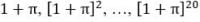 , , …, , where  is a fixed adjustment rate.

 

Exhibit 1: Cash flows of a bond ladder and a straight bond Vertical scale (in dollars) is arbitrary.] Maximum Withdrawal Rate

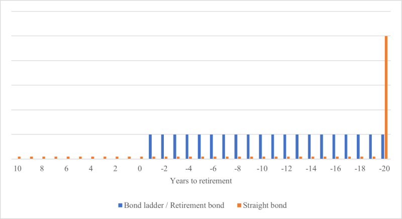
Vertical scale (in dollars) is arbitrary.

 

Maximum Withdrawal Rate

In the absence of arbitrage opportunities, the bond price is the sum of future discounted cash flows, that is

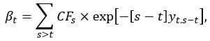
where summation is over cash flow dates posterior to t and  is the nominal zero-coupon yield of maturity . If the retirement time is conventionally denoted as time 0, the number of bonds that a newly retired individual can purchase with the retirement nest egg  is  . It can be shown that, still in the absence of arbitrage opportunities, this quantity is the maximum annual income (possibly adjusted for the cost of living) that the individual can finance. Therefore, the ratio measures the purchasing power of savings in terms of replacement income, and the maximum withdrawal rate is . It is an increasing function of interest rates since the bond price is decreasing in rates.

Exhibit 2 plots the withdrawal rate from July 1981 to January 2022 together with the yield on Treasury bonds at 10-year constant maturity. The zero-coupon yields are obtained from Data Nasdaq, which publishes a zero-coupon yield curve estimated by the methodology of Gürkaynak, Sack and Wright (2007). The figure illustrates the impact of the cost-of-living adjustment, which decreases the maximum withdrawal rate since the individual must accept lower spending in the first years in exchange for growth in subsequent years. In January 2022, the adjusted rate is 4.91%, versus 6% if no adjustment is applied. But with the 2% growth rate, adjusted withdrawals dominate the unadjusted ones after the first 10 withdrawals since

 

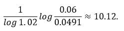
Exhibit 2: Maximal withdrawal rate.

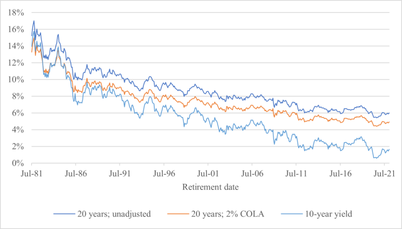
The maximal withdrawal rate is the percentage of wealth at retirement time that can be withdrawn every year for 20 years beginning one year after the retirement date. Annual withdrawals are constant in nominal terms – which corresponds to a 0% adjustment –, or subject to a 2% annual adjustment for the cost of living. The 10-year yield is the market yield on US Treasury securities at 10-year constant maturity from the Federal Reserve.]

 

Therefore, applying a cost-of-living adjustment is essentially equivalent to accepting lower consumption today in exchange for higher consumption in the future.

 

“Maximally Moderate” Spending Rule

We now describe a withdrawal rule that can be associated with any investment policy and addresses two concerns about the 4% rule, namely its uncertain feasibility and its inefficient use of resources.

Feasibility and Exhaustivity Criteria

Since the set of spending rules is virtually infinite, we first narrow down the choice by specifying desirable properties that should be satisfied. The most important requirement is feasibility, the ability to preserve a nonnegative balance of savings throughout retirement. It is the primary concern behind the design of the 4% rule, since the 4% rate was proposed by Bengen (1994) after simulating strategies with fixed withdrawals for various retirement years from 1926 to 1976 and noting that 4% withdrawals had always been sustainable for at least 30 years. This “historical method” to estimate withdrawal rates was introduced by Bierwirth (1994) as an alternative to the “average method”, which calculates them by projecting constant investment returns and inflation rates in the future. To the credit of this approach, it relies on actual scenarios rather than hypothetical scenarios with average returns and inflation, and it explicitly considers periods that were extremely unkind to retirees because of a combination of negative stock returns and high inflation, e.g. in 1973-74. Nevertheless, the historical method is subject to the same limits as any study that extrapolates past data to model the future. These concerns are expressed by Pfau (2012), who argues that the 4% rate is driven by the real returns on equities and bonds in the US over the 20th century, but the fact that these returns were higher than in other developed countries raises questions about their persistence (see also Dimson, Marsh and Staunton (2004)).

Whether the 4% rule is feasible or not in the future, it should be acknowledged that it fails to meet the exhaustivity criterion, which is the property of a strategy that does not leave any unspent surplus. Surpluses are less a problem than deficits, but they still reveal inefficiency in the use of retirement savings because they represent a missed opportunity to spend more. They implicitly appear in Bengen’s (1994) results, since there are many scenarios in which 5% withdrawals were feasible for 30 years, and even a decent number of them in which 6% was affordable. Being calibrated to the worst-case scenarios, the 4% rate is inevitably too conservative in others. The maximum withdrawal rate in Exhibit 2 addresses this concern by allowing for dependence with respect to market conditions.

 

An Alternative Spending Rule

To make fixed withdrawals corresponding to the withdrawal rates in Exhibit 2, a retiree must purchase retirement bonds and spend the cash flows. This spending-and-investment policy ensures feasibility and exhaustivity, but in a context of low rates, many individuals may find the fixed income too low to support the lifestyle they desire. Going back to Scott, Sharpe and Watson’s (2009) point that “[s]upporting a constant spending plan using a volatile investment policy is fundamentally flawed”, these retirees must accept time variation and/or uncertainty in spending if they do not follow the non-volatile investment policy, which would be 100% in retirement bonds, and target a zero final account balance.

In a 2014 article, M. Barton Waring and Laurence B. Siegel introduced a time-varying spending rule called “annually recalculated virtual annuity”, in which the withdrawal in a given year equals current savings divided by the price of a Treasury inflation-protected bond ladder with a maturity equal to the remaining horizon. In our notation, this rule says that the withdrawal in year t is

where  and  denote savings and the retirement bond price just before the withdrawal, and  includes any cost-of-living adjustment. Implicit in this specification is the constraint that the withdrawal dates match the bond’s cash-flow dates.

 

Properties

It is straightforward to see that the above spending rule is feasible and exhaustive. Feasibility follows from the fact that the pre-cash flow bond price,  , includes the current cash flow,  , so the retiree never attempts to withdraw more than the available stock of savings. At the last cash flow date, the pre-cash flow price reduces to the cash flow, so the last withdrawal consumes any remaining savings, which is the definition of exhaustivity.

The feasibility and exhaustivity conditions do not narrow down the set of admissible spending rules to a single item, and they leave the possibility of intuitively unreasonable rules, such as one that would consume all savings in the first year or one that would consume nothing until the last year and would then spend whatever is found in the portfolio. Both are feasible and exhaustive, but they lead to many years with a zero withdrawal, which is unacceptable from a retiree’s perspective.

One way to rule out such policies would be to specify a welfare criterion that penalizes very low withdrawals and pick the optimal rule with respect to that metric[M3] . We do not pursue this route to avoid the vast debate on how to model individual preferences, and because the problem of calculating optimal consumption policies has largely been addressed in the literature since the seminal work of Paul A. Samuelson and Robert C. Merton in 1969 and 1971. In a nutshell, consumption strategies that maximize a utility function have been shown to depend, among other parameters, on a risk aversion number and on state variables characterizing business conditions, such as risk premia (Merton, 1973). This dependence makes them difficult to implement in practice because risk aversion and time-varying risk premia are not easily estimated.

The spending rule that we propose has no claim to optimality with respect to any criterion, but it satisfies a few interesting properties. In addition to being feasible and exhaustive, it is moderate in the sense that the purchasing power of savings just after the withdrawal, as given by the ratio  , is never less than the purchasing power just before,  . Among all moderate rules, ours is maximal because the withdrawal  is the largest that is compatible with the moderation condition. These properties can be verified with simple calculations, using the fundamental equalities . For these reasons, we call this rule the “maximally moderate rule”.

It is worth noting that the maximally moderate rule coincides with the utility-maximizing policy when risk aversion is infinite. Indeed, Munk and Sorensen (2004) show that in this case, the optimal investment strategy is to purchase an “annuity bond” that pays a constant cash flow and is a continuous-time version of the retirement bond, and to spend a constant amount given by . When savings are invested in the retirement bond, this ratio equals the current purchasing power,  .

 

Investment Strategies Using Retirement Bonds

Strategies that are not fully invested in the retirement bond create time variation in maximally moderate withdrawals. They are advisable for individuals who find that the purchasing power of the nest egg in terms of replacement income at the retirement time is too low to support the desired lifestyle, because the inclusion of an asset class with a greater expected return than bonds, e.g. equities, creates opportunities for income growth. In this section, we examine the risk and the upside potential in terms of withdrawals of equity-bond strategies.

 

Balanced Funds and Target Date Funds

Balanced funds maintain a fixed equity-bond mix, and target date funds let the equity allocation decrease over time until a landing point is attained. Both are popular investment options, both in accumulation and in decumulation, and target date funds have earned the status of a “qualified default investment alternative” (QDIA) since the passage of the Pension Protection Act in 2006. Without going through a detailed review of the economic justifications and the limits of these weighting schemes, we note that a salient shortcoming of existing funds is that their bond bucket, which is said to be “safe”, is actually unsafe with respect to the income production objective because it does not have a duration that matches that of the retirement bond. This observation motivates the focus on balanced funds and target date funds in which the standard bond is replaced with the retirement bond.

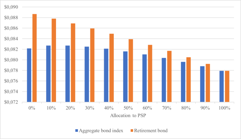
In detail, we consider balanced funds invested in an equity performance-seeking portfolio (PSP), which tracks the performance of the Scientific Beta Long-Term Track Record cap-weighted index, and a bond portfolio that replicates either the Bloomberg US Aggregate Bond index or a retirement bond. To consider various market conditions, we use the historical approach of Bierwirth (1994) and Bengen (1994), dividing our sample dataset, which ranges from July 1981 to December 2021, into overlapping 20-year decumulation periods with monthly start dates. (The periods beginning in January 2002 or later, for which withdrawals end after December 2021, are incomplete.) In each period, the maximally moderate rule is simulated, and the volatility of changes in withdrawals and the mean withdrawal are recorded. Exhibit 3 reports the statistics averaged across periods. The substitution has a volatility-reducing effect and a slightly positive effect on upside. As appears from Exhibit 4, it also has a favorable impact on downside risk, leading to an increase in the worst-case withdrawal and to a decrease in the maximum drawdown in withdrawals. Of course, the difference between the standard fund and the modified fund is bigger at low PSP allocations, which correspond to high bond allocations. Similar results would be obtained for target date funds.

The risk-reducing effect is mathematically explained by the following formula, which expresses maximally moderate withdrawals as a function of initial savings,  , the initial bond price,  , the total return index of the investment strategy, , and the total return index on the retirement bond, :[3]

 

Exhibit 3: Mean and volatility of withdrawals with balanced funds.

(a) Volatility of logarithmic changes in withdrawals (average across periods)

 

(b) Mean withdrawal per dollar invested (average across periods)

 

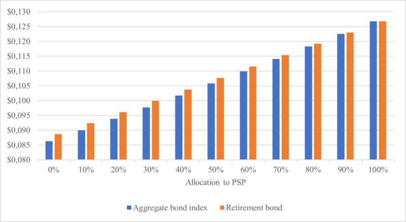
The sample is divided into overlapping 20-year decumulation periods beginning every month from 31 July 1981 to 31 December 2021. For every period, the maximally moderate rule is simulated for an individual who invests in a balanced fund made of the performance-seeking portfolio and the aggregate bond or the retirement bond. The volatility of logarithmic changes in withdrawals and the mean withdrawal are calculated across the withdrawal dates in each period and are then averaged across periods.]

 

Therefore, the volatility of changes in withdrawals and the maximum drawdown in withdrawals are identical to the tracking error and the maximum relative drawdown of the fund with respect to the retirement bond, so they are naturally lower if the fund uses a perfect retirement bond-hedging portfolio.

 

Exhibit 4: Downside risk in withdrawals with balanced funds.

(a) Minimum withdrawal per dollar invested (average across periods)

(b) Maximum drawdown in withdrawals (average across periods)

 

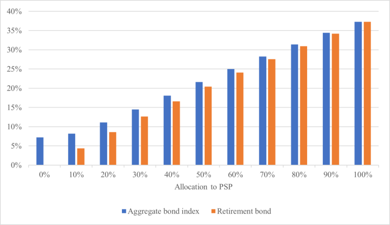
The sample is divided into overlapping 20-year decumulation periods beginning every month from 31 July 1981 to 31 December 2021. For every period, the maximally moderate rule is simulated for an individual who invests in a balanced fund made of the performance-seeking portfolio and the aggregate bond or the retirement bond. The minimum withdrawal across withdrawal dates and the maximum drawdown in withdrawals are calculated in every period and then averaged across periods.]

 

Introducing Protection Against Downside Risk

Another implication of the formula for maximally moderate withdrawals is that imposing a minimum withdrawal is mathematically equivalent to setting a floor on the relative performance of the fund with respect to the bond. Specifically, withdrawals expressed in constant dollars (the quantity   are bounded from below by the percentage δ of the initial purchasing power if, and only if, the total return of the fund in which savings are invested since the retirement time is at least δ times that of the retirement bond. This equivalence brings us back to the machinery of risk-controlled strategies to maintain a minimal fund value, when the minimum is proportional to a benchmark (here, the total return index of the retirement bond). To satisfy this constraint, Deguest et al. (2015) consider a dynamically rebalanced portfolio invested in the performance-seeking portfolio and the bond, with the following dollar allocation to the former building block:

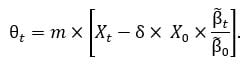
Here, m denotes a constant multiplier, like in constant proportion portfolio insurance, but a time-varying multiplier can be plugged into the formula too.

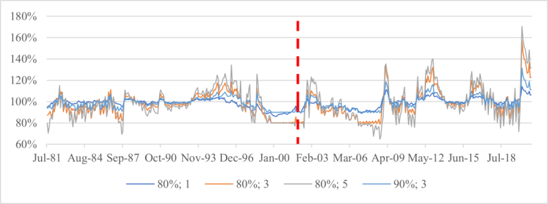
Risk control is a flexible portfolio management method that can accommodate a variety of floors, corresponding to different essential goals. The previous “constant floor” is a fixed multiple of the retirement bond index tailored to secure a fixed minimum withdrawal, but a different goal would command a different floor. For instance, if the objective is to avoid a spending cut by more than 20% with respect to the largest past withdrawal, the floor should be 80% of the past maximum value of the fund relative to the retirement bond. This “maximum drawdown floor” is

where the maximum is taken over all withdrawal dates before t, and δ = 80% in the example. A third possible floor, still of the “maximum drawdown” type, is obtained by taking the maximum over the retirement time (date 0) and the withdrawal dates up to time  , to protect a minimum amount of income and avoids spending cuts, thereby combining the advantages of the first two floors.

Exhibits 5 and 6 confirm that there is a one-to-one correspondence between an essential goal – expressed as a downside risk limit – and a floor, and that a given goal cannot be reliably attained by using a different floor. The constant floor is effective at flooring income to 80% or 90% of the initial purchasing power, except for a multiplier of 5, which causes gap risk (Exhibit 5(a)), but it opens the door to maximum drawdowns greater than 20% or 10% (Exhibit 6(a)). Conversely, the maximum drawdown floor designed to avoid spending cuts greater than 20% or 10% does avoid them for multipliers up to 3 (Exhibit 6(b)), but the worst-year withdrawal can be less than 80% or 90% of the initial purchasing power (Exhibit 5(b)). Only the third floor, which is the maximum of the previous two floors, offers protection against both risks (Exhibits 5(c) and 6(c)). For both floors, a multiplier of 5 creates gap risk, which shows up through failure to meet the downside risk constraint.

 

Conclusion

The conventional 4% rule uses a uniform spending rate that is calibrated against the worst decumulation periods, characterized by negative stock returns and high inflation, in all market conditions. As a result, it underspends the nest egg in all other scenarios, building up surpluses, and its future feasibility is uncertain because it relies on the extrapolation of conclusion drawn from past data. The first principles of asset pricing, including the absence of arbitrage opportunities, show that the maximal withdrawal rate over a period of fixed length, e.g. 20 or 30 years, is the reciprocal of a retirement bond’s price, where the retirement bond is defined as a security that pays a fixed annual cash flow of $1, adjusted for the cost of living, for the specified period. The strategy to invest in the retirement bond and to spend the cash flows addresses the problem of retirees seeking to spend their savings without outliving their assets and without running into a surplus, but it is only suitable for those who can finance the lifestyle they wish with the maximal withdrawal rate. Individuals who follow another investment policy and require an exhaustive spending policy must accept variability (over time and across scenarios) in spending. The “maximally moderate” spending rule meets the feasibility and exhaustivity conditions and leads to withdrawals that are proportional to the relative performance of the investment strategy with respect to the retirement bond. Therefore, efforts to reduce the tracking error of the strategy with respect to that bond result in less volatile withdrawals, and any cap on the relative returns of the strategy with respect to the bond translates into a floor on withdrawals.

 

The research from which this article stems was conducted as part of the EDHEC-Risk Institute/FirstRand research chair on “Designing and Implementing Welfare-Improving Investment Solutions for Institutions and Individuals”. We are grateful to Albert De Wet for very useful feedback

 

 

Footnotes

[1] In “Financial Advisors and Retirement: The Decumulation Dilemma”. PIMCO Insight. October 28, 2019

[2]  In “Tackling the ‘Nastiest, Hardest Problem in Finance’”. Bloomberg Opinion. June 5, 2017.

[3] The total return is defined as the return on the bond, with coupons reinvested in the bond as they are paid.

 

References

Bengen, W. P. (1994). Determining Withdrawal Rates Using Historical Data. Journal of Financial Planning, 7(4), 171-180.

Bierwirth, L. (1994). Investing for Retirement: Using the Past to Model the Future. Journal of Financial Planning, 7(1), 14-24.

Deguest, R., Martellini, L., Milhau, V., Suri, A., & Wang, H. (2015). Introducing a Comprehensive Risk Allocation Framework for Goals-Based Wealth Management. EDHEC-Risk Institute Publication.

Dimson, E., Marsh, P., & Staunton, M. (2004). Irrational Optimism. Financial Analysts Journal, 60(1), 15-25.

Gürkaynak, R. S., Sack, B., & Wright, J. H. (2007). The US Treasury Yield Curve: 1961 to the Present. Journal of Monetary Economics, 54(8), 2291-2304.

Kobor, A., & Muralidhar, A. (2018). How a New Bond Can Improve Retirement Security. Retirement Management Journal, 7(1), 16-30.

Martellini, L., Milhau, V., & Mulvey, J. (2019). "Flexicure" Retirement Solutions: A Part of the Answer to the Retirement Crisis? Journal of Portfolio Management, 45(5), 136-151.

Merton, R. C. (1971). Optimal Consumption and Portfolio Rules in a Continuous-Time Model. Journal of Economic Theory, 3(4), 373-413.

Merton, R. C. (1973). An Intertemporal Capital Asset Pricing Model. Econometrica, 41(5), 867-887.

Merton, R. C. (2014). The Crisis in Retirement Planning. Harvard Business Review.

Merton, R. C., & Muralidhar, A. (2017). Time for retirement ‘SeLFIES’? Investment and Pensions Europe.

Munk, C., & Sorensen, C. (2004). Optimal Consumption and Investment Strategies With Stochastic Interest Rates. Journal of Banking & Finance, 28(8), 1987-2013.

Muralidhar, A., Ohashi, K., & Shin, S. (2016). The Most Basic Missing Instrument in Financial Markets: The Case for Bonds for Financial Security. Journal of Investment Consulting, 17(2), 34-47.

Pfau, W. (2012). An International Perspective on Safe Withdrawal Rates: The Demise of the 4 Percent Rule? Journal of Financial Planning, 23(12), 52-61.

Samuelson, P. A. (1969). Lifetime Portfolio Selection by Dynamic Stochastic Programming. Review of Economics and Statistics, 51(3), 239-246.

Scott, J. S., Sharpe, W. F., & Watson, J. G. (2009). The 4% Rule -- At What Price? Journal of Investment Management, 7(3), 31-48.

Siegel, L. B., & Waring, M. B. (2015). The Only Spending Rule Article You Will Ever Need. Financial Analysts Journal, 71(1), 91-107.

 

 

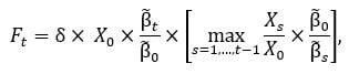
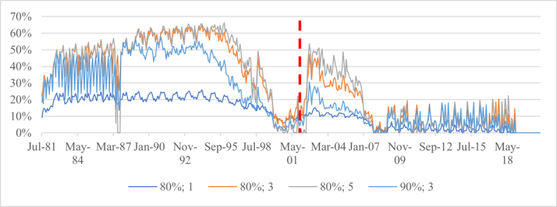
Exhibit 5: Minimum withdrawal relative to initial purchasing power.

(a) Constant floor (Floor 1)

(b) Maximum drawdown floor (Floor 2)

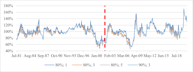
(c) Maximum drawdown floor (Floor 3)

For each monthly retirement date from 31 July 1981 to 31 December 2020, risk-controlled strategies are simulated with various floors and a multiplier of 1, 3 or 5. The parameter δ in the floor definition is 80% or 90%. Withdrawals are simulated for an individual who follows the maximally moderate rule, and the minimum withdrawal over the decumulation period is recorded and expressed as a percentage of the purchasing power of savings at the retirement time. Each date of the horizontal axis is a retirement time, and the vertical line at 31 December 2001 is the start of the last complete decumulation period.

 

 

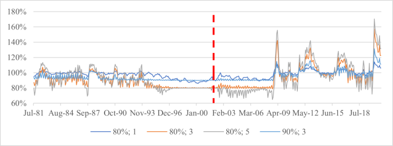
Exhibit 6: Maximum drawdown in withdrawals.

(a) Constant floor (Floor 1)

(b) Maximum drawdown floor (Floor 2)

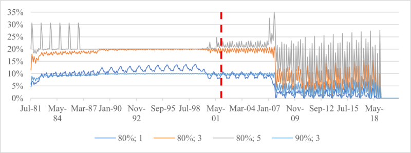
(c) Maximum drawdown floor (Floor 3)

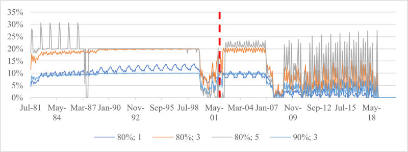
For each monthly retirement date from 31 July 1981 to 31 December 2020, risk-controlled strategies are simulated with various floors and a multiplier of 1, 3 or 5. The parameter δ in the floor definition is 80% or 90%. Withdrawals are simulated for an individual who follows the maximally moderate rule, and the maximum drawdown in withdrawals over the decumulation period is recorded. Each date of the horizontal axis is a retirement time, and the vertical line at 31 December 2001 is the start of the last complete decumulation period.

 

 

.