Including climate risks in infrastructure asset valuation: A data-driven modelling approach

In this paper we show how it is possible to include climate risks in the projections of the value of infrastructure companies at the horizon 2050, under several climate scenarios.

Introduction

Climate change is one of the most pressing challenges facing humanity today, with potentially severe implications for infrastructure assets. Infrastructure investments such as roads, bridges, ports, airports and power plants have long lifetimes, typically spanning several decades, and are designed to operate under specific climatic conditions. However, climate change is causing more frequent and intense extreme weather events, such as floods, droughts, heatwaves and storms, which can damage or disrupt infrastructure assets. These physical risks can lead to direct losses, increased maintenance costs and lower asset values. Beyond physical risks, climate change also generates transition risks, such as changes in policy, technology and consumer preferences that can impact the value of infrastructure assets. It is thus essential for infrastructure investors and other stakeholders to take climate risks into consideration when evaluating the future value of infrastructure assets. Making the economy of those could lead them to poor and high-risk decisions. Comprehensive methodologies for assessing climate risks in infrastructure asset valuation are still lacking. This article marks an important step forward in this direction: building on previous work, we develop a model that intertwines financial and macro-economic variables with Network for Greening the Financial System (NGFS) scenarios to make asset-level, scenario-dependent projections until 2050 of financial indicators such as revenues, profits, discount rates and valuation.

General approach

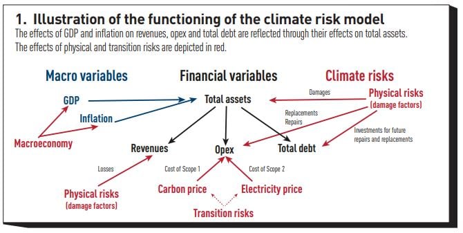
Building on previous work (Alogoskoufis et al [2021]), we first model the relationship between key financial variables in infrastructure companies (total assets, revenues, operating expenses) and macroeconomic variables (GDP, inflation). Our equations are recursive, such that variables at time t depend on the same and/or other variables at time t−1. We assume that total assets follow an auto-regressive pattern, and that their growth is correlated with GDP growth and inflation. In the infrastructure sector, we expect revenues of corporate companies to correlate with total assets. Likewise, operating expenses (opex) are expected to grow with the size (total assets) of the business. We thus regress the growth of revenues and opex against the growth of total assets. Figure 1 illustrates these dependencies. Note that the effects of GDP and inflation on revenues and opex are reflected through their effects on total assets.

After calibrating these equations, assuming that the relationships between financial and macroeconomic variables hold in the future (until 2050 at least), we are thus able to project financial variables over time, provided that we have projections of GDP and inflation. This is where the NGFS comes into play, by providing the latter for six distinct climate scenarios (the so-called ‘NGFS scenarios’) with different levels of expected climate risks. On top of macroeconomic forecasts, expected damages (physical risks) and additional costs related to the price of carbon and electricity (transition risks) must be considered when forecasting financial variables. Damages will negatively affect total assets and subsequently revenues (loss of production capacity) and increase the operating expenses through additional repair and replacement costs. On the other hand, carbon taxes to limit climate-related damages will increase the price of carbon and electricity, and thereby companies’ operating costs. All these effects are depicted in red in figure 1. Dedicated teams at EDHECinfra & Private Assets are in charge of estimating asset-level carbon emissions and expected damages. We assume that Scope 1 and 2 emissions grow at the same rate as global emissions (per country), provided by NGFS. Likewise, we get projections of carbon and electricity prices from NGFS. As for physical risks, we assume that they grow at a rate consistent with literature on floods and other risks.

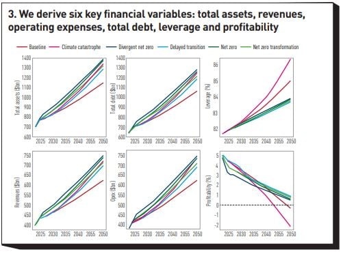
We project the total debt of companies by assuming that they keep the same capital structure over time. Total debt thus follows the growth rate of total assets. However, companies need to raise funds to cover potential future damages to total assets. Total debt thus grows faster than total assets, leading to increasing leverage. From the knowledge of total assets, revenues and opex, we can also project the profits of firms. Overall, we are thus able to generate time series until 2050 of six key financial variables (total assets, revenues, operating expenses, total debt, leverage and profits), which are then used as inputs of EDHECinfra & Private Assets’ asset pricing models to produce asset-level financial indicators such as discount rates, dividend and valuation.

Data

Financial data: infraMetrics

InfraMetrics comprises data for 7,608 companies across 33 countries worldwide. The core of our model involves linear regressions (see below) which require historical data on total assets, revenues and opex. After excluding data anterior to 2000 we have:

• Total assets: 44,584 observations across 5,589 companies and 25 countries;
• Revenues: 22,915 observations across 3,045 companies and 25 countries;
• Opex: 10,667 observations across 819 companies and 24 countries.

Macroeconomic data: World Bank and NGFS-NiGEM

For its calibration part, we feed our model with GDP and inflation data from the World Bank. For its projection part, we use climate scenario projections of the same macroeconomic variables, provided by the NiGEM model in the NGFS database.

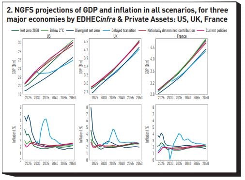
Figure 2 shows the projections of GDP and inflation for three major economies tracked by EDHECinfra & Private Assets: US, UK and France. Green, blue and red are used for orderly, disorderly, and hot house world scenarios, respectively. We see that economies continue growing relatively fast in all scenarios. Differences between scenarios exist, however, with GDP being significantly lower in the disorderly scenarios (blue lines) than in other scenarios. Similarly, inflation is particularly affected in disorderly scenarios (blue lines), highlighting the inflationary effects of stringent carbon policies. In the absence of compelling climate policies (hot house world scenarios: red lines), inflation is projected to remain relatively stable over time.

Emissions data: transition risks

One measure commonly undertaken to mitigate carbon emissions is to increase their price through a carbon tax. Such a tax directly affects the price of Scope 1 emissions through the price of carbon, and indirectly the price of Scope 2 emissions through the price of electricity (itself affected by the price of carbon). These two aspects translate into operating costs that we include in our model. We thus need, in order to project these costs, projections of Scope 1 and 2 emissions, as well as projections of carbon and electricity prices. While the latter are provided by NGFS, a dedicated EDHECinfra & Private Assets team is in charge of calculating various metrics of carbon emissions at company level, Scope 1 and 2 in particular (Nugier and Marcelo [2022]). To project these emissions into the future, we assume that Scope 1 and 2 emissions grow at the same rate as global emissions (per country), provided by NGFS as well.

Damage data: physical risks

Another dedicated team at EDHECinfra & Private Assets is in charge of estimating the impact of climate change-driven hazards on physical assets. This impact is quantified, for any single company, by a damage factor D, which represents the fraction of the area covered by the company that would be ‘destroyed’ upon the occurrence of a given hazard. Damage factors are calculated from the probability of occurrence and the intensity of various hazards in the zone where a firm is located. As of now, our calculations integrate floods, storms and cyclones as 1 in a 100-year event. That is, the probability of their occurrence is r = 1%. Importantly, D and r are calculated as of today, and are thus not scenario- or timedependent. They are, however, expected to change (and likely increase) in scenarios where efforts to mitigate climate change are insufficient.

NGFS scenarios assume that climate goals are met (ie, physical risks are mitigated, and the temperature rise remains below 2ºC) in the orderly and disorderly scenarios. Following this assumption, we thus assume that D and r remain constant in those four scenarios. In the hot house world scenarios, however, climate goals are not met, and the global mean temperature increase is expected to exceed 3ºC in the current policies scenario, and to be about 2.6ºC in the NDC scenario (NGFS [2022]). Recent research has shown that river flood damage in Europe could rise by a factor of about 6 ± 2 by the end of the century, in the absence of climate mitigation (ie, an expected 3ºC GMT increase – Dottori et al [2023]). This is consistent with a growth of about 2.3 ± 0.5% per year until 2100. Consistently with these numbers, we thus assume that D and r grow by 2% per year in the NDC scenario (2.6ºC GMT increase), and 2.5% in the current policies scenario (3.2ºC GMT increase).

Key results and conclusions

Our approach allows time series of six key financial variables to be derived: total assets, revenues, operating expenses, total debt, leverage, profitability (figure 3). Our results consistently show a downtrend in profitability in all scenarios, indicating that the implications of climate change on infrastructure companies are unavoidable. While the amplified intensity and frequency of hazard events (physical risks) will increase the costs of companies through maintenance and repairs, carbon taxes to limit these risks will increase the cost of companies’ carbon emissions (transition risks). However, scenario analysis suggests that this downward slide can be partially mitigated if immediate and coordinated action is taken by companies and governments alike (orderly scenarios). Any delay in response (delayed transition), or a lack of coordination (divergent net zero) in implementing sustainable practices will lead to transition costs that can be hard to bear, in fossil-fuel reliant sectors in particular. On the other hand, inaction (hot house world scenarios) is not a viable alternative: while it may hold off the transition costs in the near term, it will undoubtedly result in exorbitant costs in the longer run due to amplified physical damages and insurance premia.

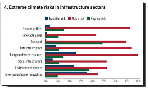
The above financial variables are then injected into the EDHECinfra & Private Assets asset pricing model to produce asset-level financial indicators such as discount rates, dividend and valuation. Knowing the values of infrastructure assets at different horizons in the six NGFS scenarios gives us the opportunity to compare projections across scenarios and thus derive metrics of climate risk. In particular, the difference in valuation between scenarios gives us measures of the potential losses incurred from transition or physical risks:

• Extreme macro risk: difference in the valuation of a company between the current policies scenario (lowest transition risks) and the delayed transition scenario (highest transition risk). While this metric, which compares two scenarios, gives a sense of the impact of making certain climate decisions or not, it forbids a direct comparison of transition and physical risks, since both are included together with a given scenario projection. To isolate and better compare the effects of either transition or physical risks, we can switch on or off the corresponding exposure terms in our model, within a given scenario:
• Extreme physical risk: within the current policies scenario (highest physical risks), difference in the valuation of a company between the case when both physical and transition risks exposures are switched off, and the case when only transition risks exposures are switched off.
• Extreme transition risk: within the delayed transition scenario (highest transition risks), difference in the valuation of a company between the case when both physical and transition risks exposures are switched off, and the case when only physical risks exposures are switched off.

We can then look at the distribution of this metric across sectors (figure 4).

References

Alogoskoufis, S. et al (2021) ECB economywide climate stress test: Methodology and results. ECB Occasional Paper Series

Dottori, F., L. Mentaschi, A. Bianchi, L. Alfieri and L. Feyen (2023) Cost-effective adaptation strategies to rising river flood risk in EuropeNature Climate Change 1–7 NGFS (2022). NGFS scenarios for central banks and supervisors Network for Greening the Financial System Nugier, F., and D. Marcelo (2022) Estimating Carbon Footprints of Transport Infrastructures Globally: the Case of Airports. EDHECinfra Research Publication