Predicting Risk Premia for Treasury Bonds: The ERI Risk Premium Monitor

Feature

Predicting Risk Premia for Treasury Bonds: The ERI Risk Premium Monitor

Riccardo Rebonato

EDHEC-Risk Institute and EDHEC Business School

October 2, 2017

Why Risk Premia Matter

Investors in the Treasury market often observe an upward-sloping yield curve[1]. This means that, by assuming ‘duration risk’, they can very often invest at a higher yield than their funding cost. Yet, if the steepness of the yield curve purely reflected expectations of future rising rates, no money could on average be made from this strategy. This prompts the obvious question: When does the steepness of the yield curve simply reflect expectations of rising rates, and when does it embed a substantial risk premium? The investment relevance of being able to answer these questions is clear. Take, for instance, a bond manager whose performance is assessed against a Treasury benchmark. His or her main strategic investment choices boil down to deciding whether to be long or short duration with respect to the benchmark. Knowing how well s/he is compensated for taking this duration risk is key to long-term performance. Or take a multi-asset portfolio manager. Deciding the relative portfolio weights among the different risk factors hinges in great part on the time-varying compensation attached to these different factors. In all these cases, and in many more, being able to estimate in a reliable and robust manner the risk premium attached to yields is key to successful investing. It is for this reason that the EDHEC-Risk Institute is launching the ERI Risk Premium Monitor: a robust tool to derive a state-of-the art estimation of the risk premium using market and monetary-policy information. This article goes on to explain how this task is achieved, and the theoretical underpinnings of the analytical tools used for the task.

Predicting Excess Returns

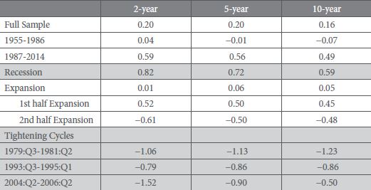
What predicts excess returns in Treasury bonds? And how much can one explain? Until recently, the answers to both questions used to be: ‘the slope’, and ‘rather little’, respectively. States of the world characterised by a steep upwardsloping yield curve used to be considered indicators of positive expected excess returns. However, the degree of predictability was modest (with R2 of the regression of the predicted and realised excess returns never exceeding 20%). To understand why the slope was deemed to be a good predictor of excess returns consider Tab (1).

Tab 1

Treasuries during the 1955-2014 period, subdivided i) into different chronological sub-periods, ii) into periods of recessions or expansions, and iii) during tightening cycles. Data adapted from Naik et al. (2016). Now, recessionary periods are associated with the monetary authorities cutting rates and therefore engineering an upward-sloping yield curve. It is also natural to assume that investors should become more risk averse in the troubled recession periods. It is therefore plausible to deduce that the yield-curve slope should explain excess returns (see, eg, Fama (1986), Stambaugh (1988), Fama and French (1989), Dahlquist and Hasseltoft (2016)). Starting from the mid-2000s, several results have questioned this received wisdom[2]: these more recent investigations suggest that different return-predicting factors may be far more complex than the simple slope[3]; and their predictions of excess returns sometimes produce much higher R2. Why is this the case? And what is the economic significance of the new, more complex, factors? Figure 1: Average excess returns from the invest-long/fund-short strategy described in the text, and the excess returns predicted by the slope and by ‘newgeneration’ return-predicitng factors (in-sample analysis, US data).

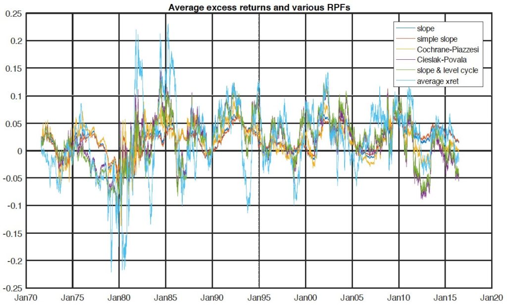 Figure 1

The motivation of the question can be readily understood by looking at Figures (1) and (2), which focus on the predictions made by the old- and newgeneration factors. More precisely, Figure (1) shows the realised average excess returns, and the excess returns predicted by the slope and other ‘new-generation’ returnpredicting factors. While all these predictions are all strongly correlated it is clear that the new-generation factors add a substantial twist to the slope story. Figure (2) makes this intuition clearer by showing the differences between the prediction produced by the slope, and the predictions produced by the newgeneration factors (in-sample analysis). Despite the fact that the new returnpredicting factors are constructed following very different prescriptions, what is added on top of the slope predictions is remarkably similar. This qualitative analysis therefore prompts the following questions:

1. Are these ‘extra predictions’ informative, or, as Bauer and Hamilton (2015) argue, are they just a result of over-fitting?
2. Why do such apparently different return-predicting factors produce such similar incremental predictions (with respect to the slope predictions)?
3. What is their financial and economic interpretation?

  Figure 2: The differences between the prediction of average excess returns produced by the slope, and the predictions produced by the new-generation factors (in-sample analysis, US data.)

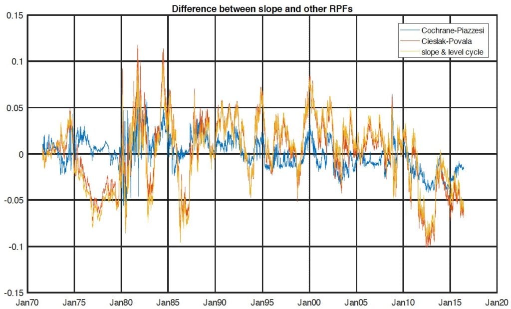Figure 2

A full answer would take too long a detour (see, eg, Rebonato (2018)). We can however summarise the main findings as follows. The first insight is linked to the power spectrum of excess returns: one can clearly see both low-frequency (business-cycle) components (well captured by the ‘old’ slope factor), but also a much higher frequency contribution, that requires higher principal components to be captured. It is (in part) because of its ability to capture these high-frequency components that a factor such as the Cochrane-Piazzesi fares better than the slope by itself. This is shown in Figs (3) (4) and (5). The first figure shows that at all investment horizons there are important contributions from both low- (‘businesscycle’) and high-frequencies components. When we look at Figs (4) and (5), which show the frequency spectrum of the slope factor and of a ‘new-generation’ factor, we note how the slope recovers the low frequency peaks of the excess returns, but completely misses the medium and high-frequency components. Contrast this with the power spectrum of the 5-year excess returns and one of modern factors, which displays a remarkable match across all frequencies. The second ‘modern’ insight alluded to above suggests that a large fraction of return predictability comes from detecting the cyclical straying of yields from a long-term fundamental trend. Once an effective decomposition of the yield dynamics into trend and cycle is carried out, one finds that the different degrees of mean reversion of the various return-predicting factors explain the different degrees of excess returns predictability very well.   Figure 3: Normalised frequency components of the power spectrum for the 2- 6- and 9-year returns. Frequencies in years−1.

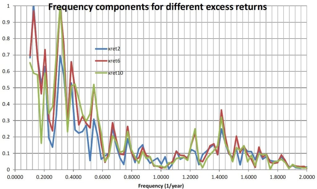Figure 3

Figure 4: Frequency power spectrum of the 2-year excess returns and of the slope return-predicting factor.

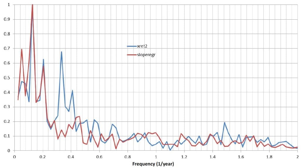Figure 4

Figure 5: Frequency power spectrum of the 5-year excess returns and of the return-predicting factor built using the slope and the cycle to the 4-years moving average of the level of yields.

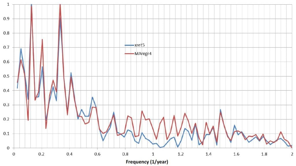Figure 5

Why do these two different ‘types of’ factors help the prediction of excess returns? We propose that two distinct financial mechanisms can explain excess returns: the first, associated with low-frequency changes in excess returns, is linked with changes in risk aversion with business-cycle periodicity. As for the second financial mechanism, associated with higher-frequency cycles, we suggest that it comes from the actions of pseudo-arbitrageurs who bring the level and slope of the yield curve back in line with fundamentals. These deviations have a much quicker mean-reversion, and are therefore associated with the higher-frequency components of the excess return spectrum. The full picture is more complex, but one can see the two key insights are that the frequency components of excess returns and their mean reverting properties give us a very effective procedure to construct powerful and very parsimonious return-predicting factors: in order to predict excess returns we need a good frequency match (across high and low frequencies), and a good match of the speed of mean reversion. When these two conditions are satisfied, a number of similarly (and highly) effective and robust factors can be built almost by inspection. The new factors are parsimonious (they only require one slope-like component and one cycle-like component), intuitively understandable (thanks to the financial interpretation offered above) and highly effective (both in-sample and out-of-sample they predict as well as, and often better than, the Cochrane- Piazzesi or the Cieslak-Povala Factors).  

Regularising the Statistical Information

As interesting as these results are, all predictions about risk premia gleaned from purely statistical studies suffer from two main shortcomings:

1. there is no guarantee that the risk premia thus estimated will be consistent with the absence of arbitrage;
2. no use is made of any information about the level of market yields: clearly, an estimate of, say, a −3% term premium has a different degree of ex ante plausibility depending on whether the corresponding market yield is, say, at 6% or 2%.

Traditionally, the ‘other’ route to estimating risk premia has been via the use of arbitrage-free affine term-structure models. Unfortunately, affine models do incorporate information about the level of market yields, and do ensure absence of arbitrage, but rarely do they have the flexibility to capture the rich information conveyed by the statistical analysis[4]. Both approaches are useful, but neither tells the whole truth. The ERI Risk Premium Monitor exploits the relative strengths of the two approaches and tries to overcome their weaknesses. It does so by complementing the predictions from the statistical estimate with the assessment of the risk premium coming from a member of the family of affine models described in Rebonato (2017). As state variables the chosen model uses the short rate, its own stochastic reversion level and the market price of risk[5]: where rt , θt and λt are the time-t value of the short rate, of its instantaneous reversion level (the ‘target rate’) and the market price of risk, respectively; σr, σθ and σλ are the associated volatilities: _θ P t and _λt are the reversion levels of the ‘target rate’ and of the market price of risk, respectively; and the increments dzr t , dzθ t and dzλ t suitably correlated. The model is fully specified once the initial state, r0, θ0 and λ0 is given. The reader is referred to Rebonato (2017) for the financial motivation of the model, and for a detailed description of its performance. For our purposes, the important observation is that the information about the P-measure path of the Fed funds (the ‘short rate’) comes from the forward guidance (the ‘blue dots’) provided quarterly by the Fed. See Figure (6). Figure 6: The path traced by the Fed ‘blue dots’ and the most similar path for the expectation of the P-measure path of the Fed funds.

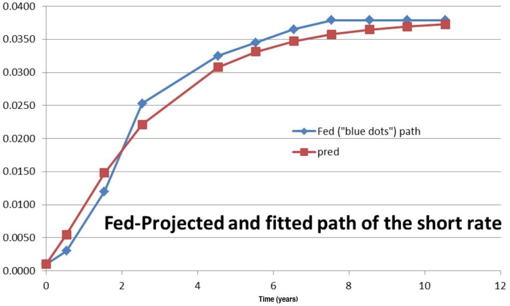Figure 6

When the two sources of information are combined, we obtain for the 10-year term premium the composite robust estimates shown in Figs (7) and (8). As Fig (7) shows, the correlation among the statistical and the model-based estimate are above 90% for all the models. This is remarkable, considering how different the approaches and the sources of information are. This congruence gives us confidence about the robustness and the reliability of the combined approach.  

Conclusions

In this article, we have given a glimpse of the latest and most exciting research strands carried out in the academic world in general, and at EDHEC-Risk Institute in particular, about the robust estimation of the yield risk premia. The predictions about the term premia for various yield maturities of the US Treasuries will be regularly provided, together with more formal research papers on these and related topics. Much work remains to be done, for instance by looking at different currencies, and at related asset classes. However, we believe that the present offering can already be of real practical use and interest for practitioners and for academics.

Figure 7: Estimates from the statistcial models and the affine model, rescaled to have the same volatility. The correlation among all the estimate is over 90%.

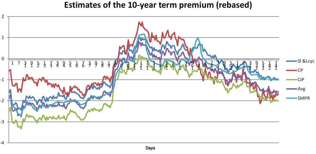Figure 7

Figure 8: The result of combining the statistical estimates of the 10-year term premium from the models in the legend combined with the estimate from the affine model.

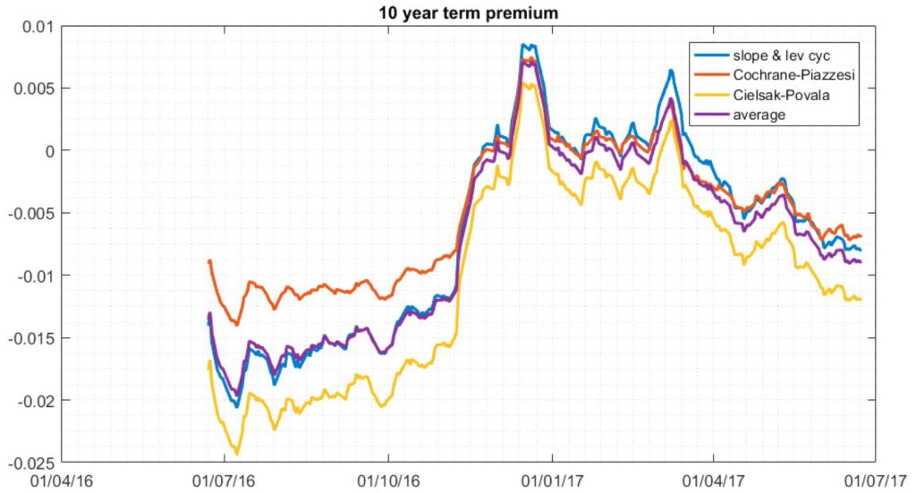Figure 8

This article is one of many articles in Investment Management Review (IMR) special edition Autumn 2017 which covers important recent insights into the asset management industry. To access the full edition please click on http://www.imrmagazine.com/edhec-special-edition.php.

[1]Since 1971, the yield curve has been upward sloping (with the 10-year yield above the 1- year yield) for almost 84% of the time. Unless investors repeatedly and erroneously expected rates to rise almost all of the time, this is prima facie evidence of the existence of a risk premium. [2]Some reference papers for the new wave of excess-return studies are Cochrane and Piazzesi (2005), Cieslak and Povala (2010a, b), Hellerstein(2011), Rebonato (2015), Dai, Singleton and Yang, (2004), Cochrane (2015). [3]For instance, the return-predicting factor of Cochrane-Piazzesi (2005) is usually referred to as a ‘tent’, and is built by giving weights of different sign and magnitude to five forward rates. In general, the common feature of the new-generation factors is that they require (implicitly or explicitly) much hihger principal components than the second — sometimes as high as the fifth. [4]This is usually because the affine dependence of the market price of risk on the state variables (required to retain tractability) is too stylised to be quantitatively useful. [5]To simplify the analysis, and in line with standard findings (see, eg, Cochrane & Piazzesi (2005, 2008), Adrian, Crump & Moench (2013)), the model assumes that investors only seek compensation for the uncertainty about the level of rates, which we proxy in our approach as the long-term reversion level of the reversion level.  

References

• Adrian T, Crump R K, Moench E, (2013), Pricing the Term Structure with Linear Regressions, Federal Reseve Bank of New York, Staff Report No 340, August 2008, Revised 2013, available at http://www.newyorkfed.org/research/staff_reports/sr340.pdf, last accessed 15th October, 2014
• Bauer M D, Hamilton J D, (2015), Robust Risk Premia, Federal Reserve Bank of San Francisco, working paper, September 2015, available at http://econweb.ucsd.edu/~jhamilto/bh_ last accessed 27 November 2015
• Burns A F, Mitchell W C, (1946), Measuring Business Cycles, Number burn46-1 in NBER Books, National Bureau of Economic Research
• Campbell J Y, Shiller, R, (1991), Yield Spreads and Interest Rate Movements: A Bird’s Eye View, Review of Economic Studies, 58, 495-514
• Cieslak A, Povala P, (2010a), Understanding Bond Risk Premia, working paper, Kellog School of Management, Wisconsin University and University of Lugano, available at https://www.gsb.stanford.edu/sites/default/files/documents/fin_01_11_Cie..., last accessed 5th May 2015
• Cieslak A, Povala P, (2010b), Expected Returns in Treasury Bonds, working paper, Northwestern University and Birbeck College, forthcoming in Review of Financial Studies
• Cochrane J H, (2015), Comments on “Robust Risk Premia” by Michael Bauer and Jim Hamilton, working paper, University of Chicago, November 2015, available at http://faculty.chicagobooth.edu/john.cochrane/research/Papers/bauer_hami... last accessed 27 November 2015
• Cochrane J H, Piazzesi M, (2005), Bond Risk Premia, American Economic Review, Vol 95, no 1, 138-160 — see also https://www.aeaweb.org/aer/data/mar05_app_cochrane.pdf (last accessed 25 November, 2014) for technical details, and the regression coefficients.
• Cochrane J H, Piazzesi M, (2008), Decomposing the Yield Curve, University of Chicago and NBR working paper, March 2008
• Dahlquist M, Hasseltoft H, (2016), International Bond Risk Premia, in Handobook of Fixed Income Securities, Veronesi P Editor, Chapter 9, 171-190
• Dai Q, Singleton K J, Yang W, (2004), Predictability of Bond Risk Premia and Affine Term Structure Models, working paper, Stern School of Business
• Fama E F, (1986), Term Premiums and Default Premiums in Money Markets, Journal of Financial Economics, 17, 175-196
• Fama E F, Bliss R, (1987), The Information in Long-Maturity Forward Rates, American Economic Review, 77, 680-692
• Fama E F, French K R, (1989), Business Conditions and Expected Returns on Stocks and Bonds, Journal of Financial Economics, 25, 23-49
• Gurkaynak R S, Sack B, Wright J H, (2007), The US Treasury Yield Curve: 1961 to the Present, Journal of Monetary Economics, 54, 2291-2304, data available at http://www.federalreserve.gov/econresdata/researchdata/feds200805.xls, last accessed 27 January, 2015 and 10 http://www.federalreserve.gov/pubs/feds/2006/200628/200628abs.html, last accessed 20 September, 2014
• Hellerstein R, (2011), Global Bond Risk Premiums, Federal Reserve Bank of New York Staff Report no 499, June 2011
• Rebonato R, (2017), Affine Models with Stochastic Market price of Risk, International Journal of Theoretical and Applied Finance, Vol 20, No 4, June, 1750027—1-1750027—38
• Rebonato R, (2018), Bond Pricing and Yield Curve Modelling — A Structural Approach, Cambridge University Press, Cambridge, UK
• Rebonato R, (2015), Return-Predicitng Factors for US Traesuries: On the Similarity of ‘Tents’ and ‘Bats’, International Journal of Theoretical and Applied Finance, Volume 18, Issue 04, 1-14
• Shiller R J, (1979), The Volatility of Long-term Interest Rates and Expectations Models of the Term Structure, Journal of Political Economy, vol 87, no 61, 1190-1218
• Stambaug R F, (1988), The Information in Forward Rates: Implications for Models of the Term Structure, Journal of Financial Economics, 22, 613-652
• Villegas D, (2015), Bond Excess Returns Predictability and the Expectation Hypothesis, thesis submitted in partial fulfillment of the requirements for the M.Sc. in Mathematical Finance, University of Oxford, Hillary Term, 2015