The Retirement Bond: How a Dedicated Safe Asset Can Help with Retirement Planning

 

Decumulation – the process of turning capital into income – has been recognized as a most difficult task, as perhaps best emphasized by strong statements made by two recipients of the Nobel Prize in economics. Richard Thaler describes it as a “more difficult challenge than accumulation”[1], while William Sharpe calls it the “nastiest, hardest problem in finance”.[2] The core difficulty is the tradeoff between current and future consumption: spending more today means saving less and thus reducing future consumption, that is unless strong portfolio performance makes up for the higher withdrawal. In brief, the decumulation problem is essentially about finding a spending rule and an investment strategy that support the desired lifestyle for as long as needed. Such decisions are complex because they must be made in the face of uncertain future returns on retirement savings and an uncertain planning horizon.

A popular approach to this problem is the so-called “4% rule”, which was analyzed by Bengen (1994) and recommends that a retiree should spend an amount equal to 4% of her initial savings plus an inflation adjustment every year. Specifically, Bengen (1994) finds that such withdrawals are sustainable for at least 33 years for individuals holding 50% or 75% of their assets in stocks and the rest in bonds, and regardless of the choice of the retirement date from 1926 to 1976.[3] The “Trinity study” by Cooley, Hubbard and Walz (1998) confirms these results and emphasizes that a substantial allocation to equities, greater than 50%, is needed to support a 4% withdrawal rate adjusted for inflation for 30 years. A series of follow-up papers have sought to improve the 4% rule by allowing for flexibility in withdrawals. For instance, Bengen (2001) lets withdrawals increase more slowly than inflation after the age of 75, and Guyton (2006) proposes to forgo adjustment for inflation after a year of negative portfolio performance. These rules allow for higher withdrawals in the early years of retirement than the 4% rule does, at the expense of lower withdrawals in later years.

Spending rules of the “x%” type seem to make retirement planning extremely simple because they establish a one-to-one relationship between a level of income and a level of wealth. For instance, according to the 4% rule, an individual should build a nest egg equivalent to 25 times the targeted real annual income. But as simple as it is, this rule of thumb creates confusion between a wealth goal and an income goal, although the latter is the ultimate objective of retirement investing and the two goals are not equivalent (Merton, 2014). That income is the quantity of interest to savers has recently been acknowledged in the US pension regulation, with the passage of the Setting Every Community Up for Retirement Enhancement (SECURE) Act in 2019. Section 105 requires administrators of defined-contribution pension plans to provide “lifetime income illustrations”. Unlike any “x%” rule, the Interim Final Rule published in August 2020 states that these illustrations should be based on an estimate for an annuity price, and it reviews assumptions (including notably longevity and interest rates) recommended to calculate that price.[4]

In contrast, the 4% rate is not based on any observed or estimated price for annuities or bonds. While the 4% rule happens to be feasible in backtests based upon US data, it suffers from several severe shortcomings. On the one hand, Scott, Sharpe and Watson (2009) point out that it involves a strong opportunity cost in the sense that it often leads to large final surpluses, suggesting that withdrawals could have been higher. They also show that by purchasing an inflation-indexed bond ladder with 30-year maturity at a 2% yield to maturity, an individual could enjoy a higher withdrawal rate of 4.46% without bearing any shortfall risk or running into a final surplus. On the other hand, Pfau (2010) shows that the 4% policy would have frequently failed in 13 out of 17 developed non-US countries from 1900 to 2008 and questions its future sustainability in the US, arguing that past good equity performance may not repeat itself. Overall, the fact that 4% is too conservative a rate in many 30-year periods and might be too high in some others suggests that an appropriate withdrawal rate should depend on market conditions, as opposed to being a “universal” value supposed to work at any point in time.

To find the maximal withdrawal rate in a given period of specified length (e.g., 20 or 30 years after the retirement date), one can use Scott, Sharpe and Watson’s (2009) bond ladder as well as the closely related concepts of “bonds for financial security” developed by Muralidhar, Ohashi and Shin (2016), “retirement SelFIES” (Standard of Living indexed, Forward-starting, Income-only Securities) by Merton and Muralidhar (2017) and “retirement bond” by Martellini, Milhau and Mulvey (2019). The retirement bond is defined as a security that pays an annual cash flow of $1 (with a possible cost-of-living adjustment) for a predetermined period. As argued below, in the absence of arbitrage opportunities, this definition implies that the maximal spending rate is the reciprocal of the bond price. Since it is a function of interest rates, the maximal rate depends on observable market conditions through the yield curve but avoids any dependency with respect to unobservable or implied parameters such as the volatilities and risk premia of risky assets. The rest of this article presents the retirement bond in more detail and explains how the maximal withdrawal rate is calculated.

 

The Safe Asset: The Retirement Bond

Conventional financial advice is for retirees to hold a mixture of stocks and bonds, with the aim of diversifying their portfolio and taking advantage of both the lower volatility of fixed income and the stronger performance potential of equities. A look at the equity glide paths of target date funds suggests that the volatility reduction objective is given priority, especially when approaching retirement. According to Morningstar’s 2018 Target-Date Fund Landscape, the equity allocation in commercial target-date funds after the target date is less than 50% and can be as low as 20% for the most conservative funds. It can be noted that, according to the results of Cooley, Hubbard and Walz (1998), such allocations do not support a 4% withdrawal rate for 30 years in all scenarios. Indeed, Cooley et al. (1998) show that a portfolio fully invested in bonds has only a 20% chance of supporting a 4% withdrawal rate adjusted for inflation for 30 years, while a portfolio consisting of 75% stocks has the best success rate, at 98%. The problem seems to be exacerbated with a decreasing equity glide path, because Bengen (1996) shows that annual decreases of respectively 2% and 3% in the stock weight will reduce the safe withdrawal rate from 4.14% to 3.81% and 3.29% respectively.[5]

Whatever the exact percentage of stocks, Scott, Sharpe and Watson (2009) argue that “[s]upporting a constant spending plan using a volatile investment policy is fundamentally flawed”. But what would be a non-volatile investment policy in the context of retirement? Merton (2014) warns us that if we reason in terms of income instead of wealth, which is the correct perspective when we think about retirement, Then Treasury bills are highly unsafe although they have the lowest volatility across most asset classes. The proper way to find a risk-free portfolio is to start from the cash flows that a retiree would target, and to identify an asset that pays these exact cash flows, or alternatively to construct a “retirement goal-hedging portfolio” that replicates them.

 

Figure 1: Cash flows of a bond ladder and a straight bond

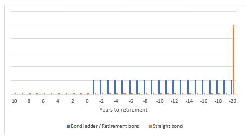
Note: Vertical scale (in dollars) is irrelevant. Only the differences between the two bonds and the variations over time are meaningful.

 

Cash Flow Schedule for the Retirement Bond

Consider an individual who is 10 years away from retirement and wants to secure fixed replacement income for the first 20 years in retirement. A 20-year period is chosen here because it approximately matches the life expectancy of a 65-year-old American. The risk-free asset for that goal is a bond ladder with equal annual payments, normalized to $1, for 20 years, beginning 10 years from now. We call this bond ladder a “retirement bond”, and its cash flows are depicted in Figure 1. It has two key characteristics: (1) a deferred start date for payments and (2) fully amortizing annual installments of equal size, achieved by progressive redemption of principal combined with interest payments. This amortization scheme is familiar to the many households that purchase real estate through a mortgage with fixed monthly payments.

Despite the name “fixed-income security”, it is important to emphasize that a straight bond does not deliver such constant cash flows. As illustrated in Figure 1, if the individual purchases a regular coupon-paying bond maturing at the end of the first 20 years of retirement, she receives coupon payments while still in accumulation when she does not need replacement income. Besides, the periodic payments are much smaller than the final one, which includes both the last coupon and the principal. As a result, there is a profound mismatch between the cash flows served by the bond and those the individual needs.

 

Inflation Indexation

The illustration in Figure 1 assumes cash flows fixed in nominal terms, of $1 per year. It is important to emphasize that over a retirement planning period that spans several decades, the impact of inflation on the purchasing power of replacement income is severe. With an average inflation rate of 2% per year – the target of the Federal Reserve and the European Central Bank –, the purchasing power of $1 is cut by one third after 21 years .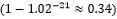

Protection against inflation can be introduced either through indexation of cash flows on realized inflation, as is done for Treasury inflation-protected securities (TIPS), or via a fixed cost-of-living adjustment (COLA), e.g. 2% per year. These options have different implications for the construction of a goal-hedging portfolio with existing Government bonds, because the former requires the use of TIPS, while the latter can be implemented with nominal bonds, which have the advantage to offer higher capacity and liquidity.

 

Measuring the Purchasing Power of Savings in Terms of Replacement Income

Retirement Bond Pricing

Just like a regular bond, a retirement bond can be priced by calculating the sum of discounted future cash flows. For cash flows fixed in nominal terms, the (dirty) price at time t, excluding the cash flow paid at that time, is given by 

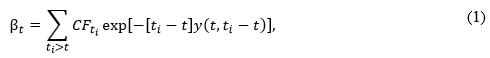
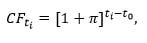
where summation is taken over all cash flow dates after time t, CFti is the cash flow of time ti and    is the continuously compounded nominal zero-coupon rate of maturity  prevailing at time ti – t prevailing at time t. This formula holds both in accumulation, i.e. before retirement, and in decumulation, i.e. after retirement. Cash flows are normalized at $1, or $1 plus a fixed compounded COLA , in which case we have

where  is a reference date for indexation.

When cash flows are indexed on realized inflation, the bond price at the reference date for indexation, , is still given by Equation (1), but nominal zero-coupon rates must be replaced with real rates.

 

Maximum Replacement Income

In the absence of arbitrage opportunities, the maximal replacement income that one can finance with the wealth level Wt  accumulated at time t, is

By letting t=0, where date 0 conventionally denotes the retirement time, it can be seen that the reciprocal of the bond price is the maximum withdrawal rate that can be sustained for 20 or 30 years, or whatever payment period is specified for the retirement bond.

Unlike any “x%” spending rule, where x is a percentage determined from historical analysis combined with a given stock-bond investment policy, the strategy that fully invests in the retirement bond and every year withdraws an amount equal to  (plus inflation or a COLA) has no risk of exhausting wealth before the bond maturity. Moreover, it makes efficient use of savings in that it leaves no unspent surplus after all scheduled withdrawals have been made. In contrast, a fixed universal rate is necessarily unsafe in some market conditions and too conservative in others. Bengen’s (1994) results show that a 5% rate is often feasible for 30 years with 50% in stocks and 50% in bonds, but there are a few periods in which it covers only 20 years of expenses,[6] so prudence calls for a 4% rate, even though 5% is likely to succeed.

To avoid incurring the opportunity cost of decreasing spending from 5% to 4%, it would obviously be desirable for the freshly retired person to know if she is at the start of a period where equity and bond returns and inflation will support 5%, or if she must make do with 4%. Since future returns and inflation are unknown, she could run Monte-Carlo simulations, taking current market conditions as initial conditions, e.g. by looking at the dividend yield to try and assess whether equities are cheap or expensive. Such simulations, however, are contingent upon assumptions about risk premia, and the corresponding estimate for the withdrawal rate will be prone to large errors. In contrast, the reciprocal of the retirement bond price provides a withdrawal rate that depends on current market conditions through discount rates but does not involve unobservable parameters such as risk premia and volatilities. The zero-coupon curve is observable, at least up to the estimation of zero-coupon rates from the market prices of Treasury securities. Gürkaynak, Sack and Wright (2007) developed an efficient estimation procedure, and their dataset is available from the website of the Federal Reserve, which we use for the calculations below.

 

Figure 2: Maximal withdrawal rate

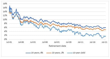
Note: The maximal withdrawal rate is the percentage of wealth at retirement that can be withdrawn every year for 20 years beginning one year after the retirement date.
Annual withdrawals are either constant in nominal terms – which corresponds to a 0% adjustment – or subject to a 2% annual adjustment for the cost of living.
The 10-year yield is the market yield on US Treasury securities at 10-year constant maturity from the Federal Reserve.

Numerical Examples

Since it is an increasing function of discount rates, the withdrawal rate has substantially reduced over the past 40 years. As evidenced in Figure 2, today’s retirees can finance much less income than those of the early 1980s per dollar saved.[7] Individuals retiring from July 1981 to July 1982 could withdraw an amount equivalent to more than 15% of their savings every year (see the “20 years; 0%” line), while those retiring in January 2022 should consume at the lower rate of 6% per year. This reduction is due to the decrease in interest rates, which can be seen for the 10-year sovereign yield in Figure 2. Note that the withdrawal rate has always been greater than the 10-year yield, and the gap between the two lines has been widening over time. One explanation is that while the yield can in principle fall to zero, the 20-year withdrawal rate must be greater than 1/20 = 5% as long as discount rates are positive.

 

Impact of Cost-of-Living Adjustment

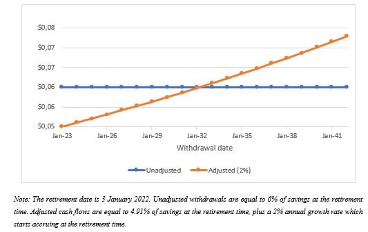
If she requires a cost-of-living adjustment, a retiree must accept a lower initial withdrawal rate. In January 2022, the rate including an adjustment of 2% per year is 4.91%, versus 6% for the unadjusted version. Because , the adjustment implies a substantial cut in spending in the first year, but after 10 years, adjusted withdrawals exceed the unadjusted ones, as can be seen from Figure 3. Therefore, applying a cost-of-living adjustment is essentially equivalent to sacrificing some consumption in the early stage of retirement for higher consumption in later years. It is up to individuals to decide whether or not their relative preference for short-term versus long-term consumption justifies such an adjustment.

 

 Figure 3: Adjusted versus non-adjusted withdrawals for $1 of savings on 3 January 2022

 

Comparison with the 4% Rule

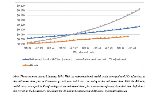
The withdrawal rates in Figure 2 cannot be directly compared with the popular 4% rate because Bengen (1994) determined this value by requiring a minimum payment period of 30 years as well as inflation-indexed retirement income cash flows. For a fairer comparison, let us consider a payment period of 30 years and apply an adjustment to proxy for expected inflation. With these parameters and a 2% annual adjustment, the maximal withdrawal rate for a person retiring on 3 January 1994, at the start of the year in which Bengen’s original paper was published, is 6.24%. This value is much greater than 4%, but one might wonder whether the adjustments for realized inflation prescribed by the 4% rule eventually lead to greater withdrawals than the 2% adjustment. Figure 4 shows that this is not the case – at least for the 27 years for which inflation data is available to date –, and also that the withdrawals with the retirement bond dominate those made under the 4% rule. Even by requiring a 5% annual growth in payments, which decreases the maximal withdrawal rate from 6.24% to 4.32%, the withdrawals with the retirement bond remain greater than those of the 4% rule. Therefore, the 4% rule led individuals who retired in the mid-1990s (at the time the paper was published) to underspend.

 

Figure 4: Withdrawals with retirement bond versus withdrawals with 4% rule for $1 of savings on 3 January 1994

 

On the other hand, a withdrawal rate of 4% may not be sustainable for 30 years with certainty in the market conditions of January 2022. With a cost-of-living adjustment of 2% per year, the maximal rate for an individual retiring on 3 January 2022 is indeed only 3.33%. We can also take advantage of a real discount curve now being available to calculate the price of a retirement bond with inflation-indexed cash flows of $1 in real terms.[8] The maximal withdrawal rate for a retiree requiring indexed cash flows is 3.05%, which is still less than 4%. This does not mean that the savings of an individual withdrawing 4% plus inflation every year beginning in January 2023 will necessarily be exhausted before the 30 years are up, but these withdrawals will only be feasible in some scenarios for equity returns and inflation. In other words, a 4% rate is literally “unsafe” in current market conditions.

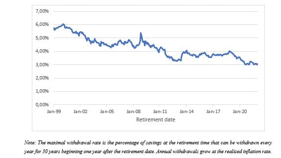
As evidenced in Figure 5, which shows the maximal withdrawal rate for an individual who targets 30 years of inflation-adjusted withdrawals, this situation has prevailed since August 2011 with a maximal rate that has ranged from 3% to 4%. Before August 2011, it used to be greater than 4%, so the 4% rule was then too conservative. In conclusion, there is simply no “universal” safe withdrawal rate that is valid at any time and in any market conditions.

 

Figure 5: Maximal withdrawal rate with inflation-adjusted withdrawals and a 30-year decumulation period

 

Today’s retirees might be disappointed that the maximal withdrawal rate for a 30-year period and inflation-adjusted withdrawals is less than the supposedly universal 4% level. This situation is due to the current environment with negative real interest rates, which makes 4% spending an aspirational goal in the terminology introduced by Deguest et al. (2015). To maximize their chances of achieving that goal, retirees must take some risk and invest part of their savings in an asset class, typically equities, that is expected to outperform the retirement bond. However, risk should be taken with caution in order not to put the retiree’s lifestyle at risk. Recent research by Martellini and Milhau (2020) suggests that the retirement bond is a helpful building block, leading to more efficient spending of investors’ risk budgets, in the context of goal-based investing strategies designed for the pre-retirement phase. Extension to the decumulation phase is the focus of ongoing research.

 

Conclusion

While the 4% spending rule and its variants have proved to be sustainable in historical backtests, there is no guarantee that they will be successful for individuals retiring now or in the future. Moreover, their sustainability is achieved at the cost of underspending in many scenarios where the retiree is left with a surplus at the end of the planning period. In this paper, we argue that a sustainable and efficient withdrawal rate should be a function of market conditions, and we show that a meaningful withdrawal rate is given by the reciprocal of the price of a “retirement bond”, defined as a bond ladder that pays $1 (possibly adjusted for inflation or the cost of living) per year for the planning period. The retirement bond price can be calculated from the observable yield curve and does not involve any subjective assumption about risk premia or the retiree’s tolerance for risk. It enables retirees to very easily calculate how much income they can generate from their retirement pot. The retirement bond itself can be regarded as the risk-free asset for those who want to secure income for a predetermined period, e.g. for the first 10, 20 or 30 years in retirement. For these reasons, the retirement bond and its price appear to be key ingredients in the design of sustainable and efficient spending and investment strategies in decumulation.

 

The research from which this article is drawn has benefitted from the support of Bank of America in the context of the research chair “Decumulation Investing: Taxonomy, Axiomatic Framework and Financial Engineering Solutions”.[9]

 

Footnotes

[1] Thaler, R., 2019. Financial Advisors and Retirement: The Decumulation Dilemma. PIMCO Insight, October 28, 2019.

[2] Sharpe, W., 2017. Tackling the “Nastiest, Hardest Problem in Finance”. Bloomberg Opinion, June 5, 2017.

[3] Because his dataset ended in 1992, Bengen used average stock and bond returns and an average inflation rate for subsequent years.

[4] The SECURE Act requires two values of income to be provided. One is obtained by converting savings into a single life annuity, and the other by converting them into a joint and survivor annuity.

[5] But Bengen (1996) finds that a 1% annual decrease in the equity allocation has no material impact on the safe withdrawal rate, which remains slightly greater than 4%.

[6] See his Figure 1(c).

[7] That withdrawal rates have been decreasing does not imply that today’s retirees have less income from their savings than those who retired in the early 1980s because, owing to inflation effects, the nest egg may be bigger today.

[8] We use the real zero-coupon yield curve estimated by Gürkaynak, Sack and Wright (2010). The updated dataset is available from the Federal Reserve website. Zero-coupon rates are available for maturities ranging from two to 20 years, but we need to discount cash flows with maturities ranging from one to 30 years, so we extrapolate the one-year rate to the left and the 20-year rate to the right.

[9] We thank Anil Suri for very useful feedback.

 

References

Bengen, W. P. (1994). Determining Withdrawal Rates Using Historical Data. Journal of Financial Planning, 7(4), 171–180

Bengen, W. P. (1996). Asset Allocation for a Lifetime. Journal of Financial Planning, 9(4), 58–67

Bengen, W. P. (2001). Conserving Client Portfolios During Retirement, Part IV. Journal of Financial Planning, 14(5), 110–119

Cooley, P. L., Hubbard, C. M., & Walz, D. T. (1998). Retirement Savings: Choosing a Withdrawal Rate That Is Sustainable. AAII Journal, 20(2), 16–21

Deguest, R., Martellini, L., Milhau, V., Suri, A., & Wang, H. (2015). Introducing a Comprehensive Risk Allocation Framework for Goals-Based Wealth Management. EDHEC-Risk Institute Publication

Gürkaynak, R. S., Sack, B., & Wright, J. H. (2007). The US Treasury Yield Curve: 1961 to the Present. Journal of Monetary Economics, 54(8), 2291–2304

Gürkaynak, R., Sack, B., & Wright, J. (2010). The TIPS Yield Curve and Inflation Compensation. American Economic Journal: Macroeconomics, 2(1), 70–92

Guyton, J., & Klinger, W. (2006). Decision Rules and Maximum Initial Withdrawal Rates. Journal of Financial Planning, 50–58

Martellini, L., Milhau, V., & Mulvey, J. (2019). "Flexicure" Retirement Solutions: A Part of the Answer to the Retirement Crisis? Journal of Portfolio Management, 45(5), 136–151