Robust and interpretable liquidity proxies for market and funding liquidity

We introduce a method to create two interpretable liquidity measures, which we associate with market and funding liquidity. The construction is based on creating two parsimonious linear combinations of the many liquidity proxies often used in the liquidity literature, both displaying mean-reverting behaviour, but characterized by very different reversion speeds. Our construction does not require transaction-level data (such as volume or bid-offer spreads), but correlates well both with other measure that do, and with other liquidity proxies (liquidity as ‘noise’, liquidity as broker-dealer leverage) recently introduced in the literature. 

 

The importance of liquidity is widely recognised by both academics and practitioners. Unfortunately, being a latent quantity, liquidity is not easy to measure (and sometimes even to define). Most proxies of liquidity require the use of microstructural, transaction-level data. This type of information is often proprietary, and, when publicly available, it often refers to the most liquid securities – for which liquidity impairment is arguably less of a problem.

This paper therefore introduces a statistical method to estimate two measures of liquidity (which we call ‘market’ and ‘funding’) with the following positive features:

• they can be calculated using publicly available prices or yields;
• they are interpretable;
• they correlate well with measures that require transaction-level data (such as the measures recently introduced by Hu, Wang and Pan [2015]; Konstantinovsky, Ng and Phelps [2016], and Adrian, Etula and Muir [2015]);
• they can be easily translated (eg, via regression) into the sensitivity to market and funding liquidity of individual securities.

The intuition behind our approach is very simple. First we identify a number of proxies whose behaviour is affected, possibly together with other factors, by changes in liquidity. We construct their covariance matrix, and carry out (sparse and traditional) Principal Component Analysis. By retaining only the first (two) principal components, we attempt to ‘push’ the nonliquidity confounding factors (such as credit) into the higher components (which we neglect). Of course, we have to justify our claim that most of the non-liquidity factors have indeed been pushed into the higher principal components that we neglect.

When we carry out this procedure, we identify two clear measures of liquidity, which we characterise as ‘market’ and ‘funding’ liquidity components. We also find that these two measures of liquidity naturally sort the input proxy variables into two distinct sets of proxies, with very different and very clearly identifiable reversion speeds, which are neatly inherited by the measures we build.

 

Market and funding liquidity

The literature on liquidity is vast (albeit strongly skewed towards equities). For a useful recent review, see Adler (2012). The contributions most closely linked to our work are Brunnermeier and Pedersen (2009), whose results are discussed later in this section; Hu, Pang and Wang (2012); Adrian, Etula and Muir (2014), and Acharya and Pedersen (2005), whose results are compared with ours in detail in the section ‘Comparison with related work’.

It is widely recognised that there are (at least) two aspects of liquidity, often referred to as market liquidity and funding liquidity, or ‘normal’ and ‘crisis’ liquidity. See Danielsson, Song Shin and Zigrand (2009) for a theoretical treatment and International Monetary Fund (2015) and Bank for International Settlements (2016) for an institutional perspective. Brunnermeier and Pedersen (2009), Danielsson, Song Shin and Zigrand (2009) and Boudt, Paulus and Rosenthal (2013), among others, have investigated the effects of these different liquidity regimes on asset prices. Despite the wide acceptance of the existence of two ‘types’ of liquidity, there is no consensus about how these two regimes or modes should be defined, let alone identified.

In our approach we do not posit a priori that there should exist one or two ‘types’ of liquidity. Rather, two different liquidity measures naturally arise from the procedure we describe below, and we argue that these two statistically-obtained measures can be clearly distinguished from one another (on the basis of their different reversion speeds). More precisely, we estimate our liquidity measures by adapting an approach first introduced by Ludvigson and Ng (2009) in the context of excess returns in US Treasuries.

We adapt and modify their procedure as follows. We first choose n financial time series, yt, each of length N, which we have reason to believe are strongly affected by liquidity (see the next section for a justification of our choices of variables). Next, as in Korajczyk and Sadka (2008), we standardise the proxies by subtracting their mean and dividing by their standard deviation. We then create the covariance matrix, Σlev, among their levels and we orthogonalise it: 

where V is the n×n orthogonal matrix of eigenvectors, and L the n×n diagonal matrix of eigenvalues. With the eigenvectors thus obtained we construct the N×n matrix of principal components,

We retain k < n of these principal components, which we interpret as liquidity measures and analyse in the ‘Comparison with related work’ section below.

 

Choice of and justification for the component proxies

Which proxies should reasonably be considered representative of liquidity (ie, how should we choose the n financial time series, yt)?

First of all, microstructural considerations (see, eg, Easley et al [2011]; Foucault, Pagano and Roell [2013], and Brunnermeier and Pedersen [2013]) and analysis of macro-financial data (see, eg, Fontaine and Garcia [2015]) suggest that liquidity should be inversely related to volatility. We therefore include volatility-related quantities in our set of input liquidity proxies.

During periods of severe market distress there is a well-documented tendency for investors to try to shift their portfolios towards safe-haven assets such as Treasuries (this is the deleveraging phase in our model). This can only be achieved by selling riskier assets. Concentrated selling pressure in these riskier assets creates problems for the associated market makers, leading to wider spreads and reduced liquidity. Therefore some indicators of preference for safe-haven assets should be included in our list of liquidity proxies. Among these, the on-the-run/off-the-run spread (difference in yields between the on-the-run and off-the-run 10-year Treasury, discussed at length in Fontaine and Garcia [2015]) is probably the ultimate safe-haven indicator, and we therefore include it in our set of proxies.

The same reorientation of portfolios away from risky assets also occurs, albeit over longer time frames, when economic fundamentals are perceived to have worsened or to be worsening. If the assets that investors want to dispose of are illiquid to start with (such as emerging market bonds or high-yield credit issues), this systematic selling pressure can also create problems for market makers, and hence reduce the liquidity of the assets. Therefore we include quantities such as emerging market and high-yield bond spreads among our proxies.

Finally, a reduction in liquidity can hinder the access to funding for the pseudo-arbitrageurs and the immediacy providers (market makers); indeed, Fontaine and Garcia (2015) find that liquidity is linked to factors measuring monetary conditions in the economy and in the banking system in particular. We therefore include quantities such as the TED and LIBOR/OIS spreads as plausible indicators of (funding) liquidity.

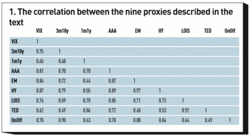
The chosen proxies are all strongly correlated (see figure 1) and each one is a very plausible proxy for liquidity. Indeed, casual inspection of their time series, as in figure 2, would make it very difficult to attribute a priori any deep meaning to the differences between any two proxies: at first blush, any or all of them could be taken as a defensible liquidity proxy. In reality we show in what follows that this superficial similarity hides subtle but important differences.

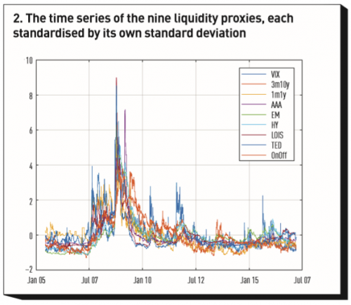
In order to quantitatively differentiate between the proxies, we examined their mean-reverting properties. The reversion speeds and half-lives of the nine proxies are shown in figure 3, sorted by increasing reversion speed. 

As this figure shows, we find a very wide range of mean reversion speeds, with half-lives ranging from two months to almost a year and a half. Since the speed of mean reversion is linked to the time over which liquidity is typically restored to the market after a shock, this is a very important quantity. We will revisit their behaviour in what follows, but for the moment we note that the two fastest mean-reverting proxies (LOIS and TED spreads) are both closely linked to the funding of financial intermediaries (dealer/brokers – the pseudo-arbitrageurs in our model).

Apart from the ability to provide a useful interpretation, this grouping of the standardised proxies on the basis of mean reversion is also quantitatively interesting, because, as we shall see, it is closely mirrored in the different reversion speeds of our two liquidity measures. 
 

Features of our liquidity measures

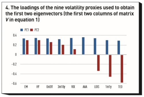
The orthogonalisation of the covariance matrix of the nine chosen proxies (see equation 1) produces the first two eigenvectors shown in figure 4. The first principal component displays the usual almost constant-loading pattern found in most principal component analyses. The second principal component is made up of positive loadings for LOIS and TED (the two fastest mean-reverting proxies, again confirming that these two variables ‘work together’) and of negative loadings for OnOff, EM and HY (all associated with the slowest reversion speeds). It is very interesting to note how the differences in reversion speeds (which the PCA ‘knows nothing about’) are exactly picked up in the construction of the loadings for the second principal component. A sparse PCA (not reported in detail for the sake of brevity) confirms this grouping. The time series of the first two principal components, PC1t and PC2t, obtained from the first two columns of the quantities PCt in equation 2 are shown in figure 5. These quantities are key to our analysis because they are our measures of liquidity. 

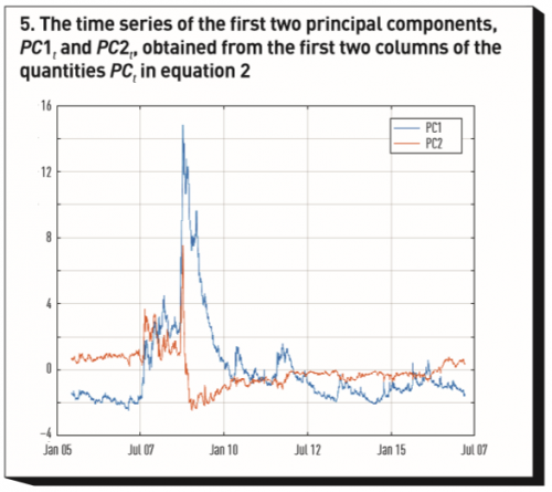
The incremental and cumulative percentage of the total variance explained by the first n principal components (n ≤ 1 ≤ 9) is shown in figure 6: we note that the first two principal components explain close to 90% of the total variance of the nine proxies, suggesting that little is lost by neglecting the higher eigenvectors.

Finally, as for the reversion-speed properties of the first two principal components, we note that the first is much more slowly mean-reverting than the second (with half-lives of 1.27 and 0.39 years, respectively, nicely mirroring the reversion speeds in figure 3). This important aspect is discussed at length in the next section, where we offer an interpretation of the two liquidity measures that we have introduced in this section. 

 

Interpretation of the liquidity measures

The market/funding interpretability of our liquidity measures is an important feature of our approach. So far we have established some empirical facts:

• that the original liquidity proxies have a wide range of reversion speeds, with funding-liquidity proxies the fastest mean-reverting; 
• that our two liquidity measures display different reversion speeds;
• that the reversion speeds of our liquidity measures closely match the fastest and slowest reversion speeds of the input proxies; and
• that the fastest-reverting proxies are associated with funding liquidity.

Therefore we make the inference that we can associate one liquidity measure with funding liquidity and the other with market liquidity. In this section we therefore explore in detail whether this inference is warranted by undertaking a detailed event analysis.

To this effect, we carry out a careful comparison of the salient features of the two principal components (such as peaks, trends, levels, etc) against major events in the period under study which can be plausibly assumed, or are known, to have had an impact on liquidity, and on the availability of funding. In figures 7 and 8 we present times series for the first two principal components, punctuated by the salient events of the period under consideration. (A description of the abbreviations and a short narrative is provided in the appendix.)

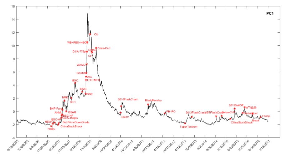
Figure 7: Time series of the first principal component, with selected salient liquidity-related market events as markers

 

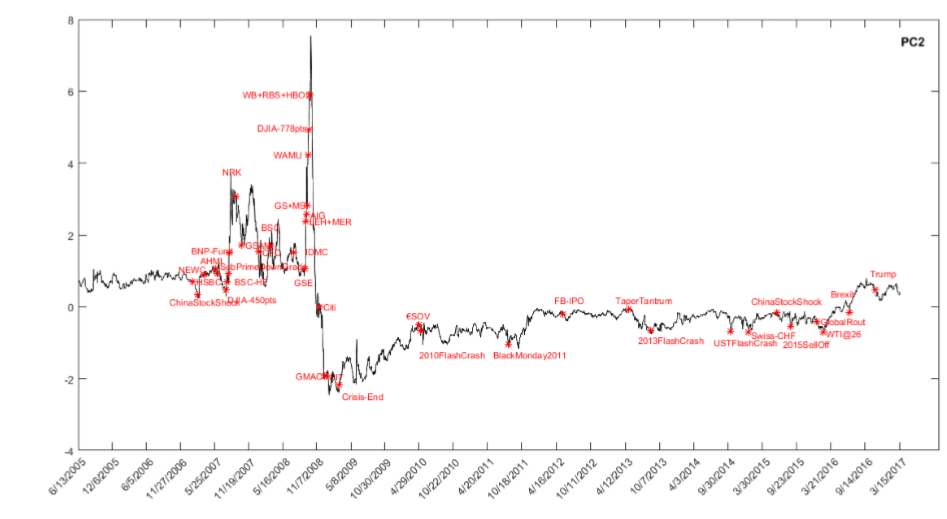
Figure 8: Time series of the second principal component, with selected salient liquidity-related market events as markers.

 

First, we note that all the major crisis events (LEH+MER, WAMU, WB, DJIA−778pts etc) have left a clear signature in the time series of both principal components as a sharp increase. Next, we note that when the second principal component peaks, the first also peaks, but the converse is not true. For instance, figure 8 clearly shows that there is a single major peak in the time series of the second principal component, located in the immediate aftermath of the Lehman default, and two minor peaks on 20 August 2007 and 12 August 2007. These peaks are all also present in the time series of the first principal component, as shown in figure 7. This latter series, however, also displays pronounced peaks on 5 March 2009, 4 October 2011, 23 November 2011, 24 August 2015 and 11 February 2016, but these peaks are not present in the time series of the second principal component. Other minor peaks are visible for the first principal component and, again, these are missing or very muted in the time series of the second principal component.

This is again consistent with the interpretation of the second principal component as an indicator of the deterioration in liquidity associated with the severest dislocations (funding liquidity shock in our model), and that of the first principal component as a reflection of all sources of liquidity deterioration.

Another feature is worth discussing. The point labelled ‘Crisis-END’ ushers in the onset of a very clear decaying exponential-like reduction in the first principal component after the end of the crisis.<a href="#_ftn1" name="_ftnref1">[1]</a> The same end-of-crisis marker corresponds to the end of the fall for the second principal component. The most significant changes associated with this marker are therefore after the end-of-crisis point for the first principal component, and before it for the second. This is consistent with our interpretation of the two principal components as market-plus-funding and funding-only liquidity indicators: as market and economic conditions progressively heal, the first principal component signals a continuous and slow improvement in market liquidity; once the severe distress is over, however, the second principal component does not signal any further improvement in the funding liquidity, despite the fact that the world economy is far from healed.

Finally, we note that changes in equity market excess returns<a href="#_ftn2" name="_ftnref2">[2]</a> are strongly (negatively) correlated with the first principal component (r = −60%), but virtually uncorrelated with changes in the second (r = 1%). This fits in well with a model like that of Brunnermeier and Pedersen (2008), who point out that market liquidity should co-move with the market factor, and with the findings in Fontaine and Garcia (2012), who find that liquidity covaries positively with changes in aggregate uncertainty, which they also proxy by the volatility of the S&P500 index.<a href="#_ftn3" name="_ftnref3">[3]</a>

In sum: the event analysis presented in this section points to the following conclusions:

• the largest deterioration of liquidity is due to the withdrawal of funding; more mundane occurrences of (market) liquidity impairment occur more frequently;
• shocks to market and funding liquidity are reversed with very different reversion speeds; and
• the reversion speeds of our two measures closely mirror the reversion speeds of market and liquidity shocks. 

Comparison with related work We have discussed at length the salient features of our liquidity measures. In the literature, a number of liquidity proxies have been recently proposed. How do they compare with our measures?

Our first observation is that the liquidity measures which have been recently introduced all require the availability of granular or aggregate transaction-level data (bid-offer spreads, volume information, broker-dealer inventories, etc). While obtaining some of the transactional data may be relatively simple for equities, it can pose serious problems for other asset classes. In this section we therefore compare our measure(s) of liquidity, which rely only on readily available price information, with the most popular measures introduced in the recent literature, all of which use additional information other than past prices. These measures are:

• ‘Liquidity as noise’ by Hu, Wang and Pan (2015)<a href="#_ftn4" name="_ftnref4">[4]</a> – Noise hereafter;
• the Barclays Liquidity Credit Score by Konstantinovsky, Ng and Phelps (2016) – LCS hereafter; 
• the broker-dealer leverage measure by Adrian, Etula and Muir (2015) – BDL hereafter; and
• Pastor and Staumbaugh’s (2003) aggregate liquidity measure – P&S hereafter.

Noise is built from the pricing errors in fitting to individual Treasuries using a popular fitting methodology (Nelson and Siegel [1987]). The intuition is that, in normal market conditions, the small price deviations from fair value (as ascertained by the Nelson-Siegel model) are arbitraged away by speculators. As market liquidity deteriorates, in the model by Hu, Wang and Pan (2015) speculators have less available capital to ‘correct’ the price deviations, which therefore become a signal of market liquidity. If our interpretation is correct, the Noise measure can therefore be expected to be more strongly correlated with our first measure, which captures both types of liquidity impairments.

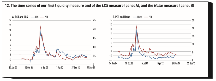
The LCS measure is built using Barclays dealer quote data<a href="#_ftn5" name="_ftnref5">[5]</a>, and is a direct trading cost expressed as a percentage of the bond price. It is bond-specific and updated daily. By the way it is constructed, it should reflect changes in both funding and market liquidity, and should therefore display the strongest correlation with our first liquidity measure.

Adrian and Etula (2015) argue that liquidity is linked to the pro-cyclical broker-dealer balance sheet adjustments. They therefore construct a measure of leverage by defining BDL as 

We independently constructed a dealer leverage factor using data from the Financial and Operational Combined Uniform Single Report (Focus). While the firms selected by Adrian and Etula (2015) were limited to primary dealers, with our data we were able to access the raw total assets and equity for over 400 US-registered broker-dealers at a monthly frequency, thereby creating a more comprehensive measure. By the way it has been constructed, we expect the BDL measure to more closely track our second principal component, which we have associated with deterioration in funding liquidity, than the first.

Finally, the P&S measure is extracted from volume-related stock return reversals cross-sectionally. Using data between 1966 and 1999 the authors found that on average 7.5% annual return can be attributed cross-sectionally to a market-wide liquidity. Sharp declines in their Aggregate Liquidity measure coincide with market downturns and flights to quality.

To explore whether our liquidity measures behave as expected, we regress the four indicators of liquidity mentioned above, LiqIndt, against our first and second principal components:

with the index k identifying the four liquidity measures found in the recent literature (k = 1: Noise, k = 2: LCS, k = 3: BDL, k = 4: P&S indicator).

Our predictions are well borne out by the results of the regressions, shown in figure 9. In particular:

• the Noise and LCS liquidity indicators are strongly correlated with our first liquidity measure, and weakly with the second;
• the BDL indicator is strongly correlated with our second liquidity measure, and weakly with the first. It is also weakly correlated with Noise and
  LCS  ; 
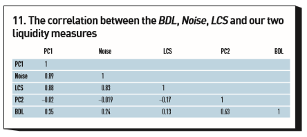
• plotting the BDL measure against Noise and LCS clearly shows that BDL picks up very different aspects of liquidity: in the initial phases of the crisis it remains elevated, suggesting, in line with Adrian and Etula (2015), strongly pro-cyclical behaviour. See figures 10 and 11, which show the correlation between the BDL, LCS, Noise, PC1 and PC2 liquidity measures.

Neither of our principal components shows any correlation with Pastor and Staumbaugh’s liquidity measure, but this measure shows little or no correlation with any of the other liquidity measures discussed in this section.

 

 

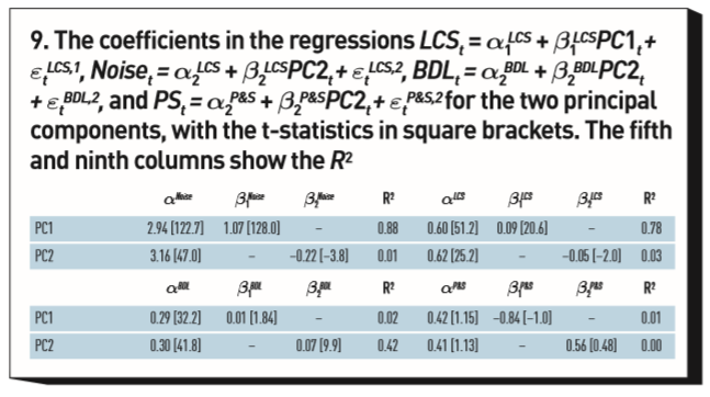
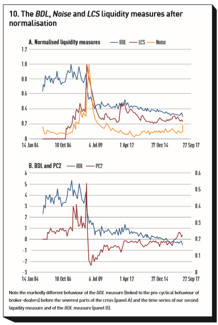
Overall, the interpretation of the first principal component as a mixture of market and funding liquidity and of the second principal component as a proxy for funding liquidity has found further corroboration from the analysis presented in this section. Given the way we have defined liquidity (market or funding) as the cost of a buy-and-sell ‘round trip’, it is also very comforting to note the close link between our first liquidity measure and the LCS measure (that is directly built using bid-offer information). This is particularly noteworthy because we do not use bid-offer or any transaction-level information in our construction.

Conclusions

This paper introduces two novel measures of liquidity, linked to what we define as ‘market’ and ‘funding’ liquidity. Our measures can be constructed using publicly available prices and yields, yet are highly correlated with recently proposed measures that require information such as bid-offer spreads, broker-dealer leverage or the output of a Treasury fitting model.

We claim that simplicity of construction is not the only (or indeed the main) positive feature of our measures. We have made the case that our liquidity measures:

• pick up different aspects of liquidity, namely market and funding liquidity (which we have defined);
• are less likely to be affected by non liquidity-related confounding factors (such as credit); and
• are interpretable.

Our two liquidity measures differ by their mean-reversion properties, highlighting fast and slow mean-reverting ‘types of’ liquidity shocks. This different behaviour is clearly mirrored in the mean-reverting behaviour of the underlying proxies. To our knowledge these differences in speeds of liquidity restoration have not been commented on before, but we think that they are highly meaningful.

 

Footnotes

[1] By 9 March 2009, the Dow had fallen to 6,440, exceeding the pace of the market’s fall during the Great Depression and reaching a level which the index had last seen in 1996. On 10 March 2009, a rally began which took the Dow up to 8,500 by 6 May 2009. By 9 May, financial stocks had rallied more than 150% in just over two months. The start of March has therefore been taken as the end point for the crisis. /p>

[2] We have taken returns on the S&P500 as a proxy for equity market returns.

[3] Fontaine and Garcia (2012) look at implied rather than realised volatility. The two quantities are highly correlated.

[4] We thank Dr Pan for providing the Noise data series.

[5] We thank Konstantinovsky, Ng and Phelps for making the BLC data available..

References

Acharya, V., and L. Pedersen (2005). Asset Pricing with Liquidity Risk. Journal of Financial Economics 77: 375–410.

Acharya, V., H. Almeida, F. Ippolito and A. Perez (2014). Credit Lines as Monitored Liquidity Insurance: Theory and Evidence. Journal of Financial Economics 112: 287–319.

Adler, D. (2012), The New Field of Liquidity and Financial Frictions. The Research Foundation of CFA Institute Literature Review.

Adrian, T., E. Etula and T. Muir (2014). Financial Intermediaries and the Cross-Section of Asset Returns. Journal of Finance 69: 2557–2596.

Adrian, T., and H. Shin (2008). Liquidity and Leverage. Federal Reserve Bank of New York Staff Reports, No 328.

Ali, A., K. Wei and Y. Zhou (2011). Insider Trading and Option Grant Timing in Response to Fire Sales (and Purchases) of Stocks by Mutual Funds, Journal of Accounting Research 49: 595–632.

Almgren, C., C. Thum, E. Hauptman and H. Li (2005). Direct Estimation of Equity Market Impact. Risk July: 57–62.

Amihud, Y. (2002). Illiquidity and Stock Returns: Cross-Section and Time-Series Effects. Journal of Financial Markets 5: 31–56.

BIS (2016). Fixed Income Market Liquidity. Committee on the Global Financial System (CGFS), No 55.

BIS (2019). BIS Global Liquidity Indicators: Methodology. Available at www.bis.org/statistics/gli/glimetho

Boudt, K., E. Paulus and D. Rosenthal (2013). Funding Liquidity, Market Liquidity and TED spreads: A TwoRegime Model. National Bank of Belgium, Working Paper No 244.

Brunnermeier, M., and L. Pedersen (2009). Market Liquidity and Funding Liquidity. Review of Financial Studies 22(6): 2201–2238.

Bullock, N. (2012). Wall Street: Inventory Reductions Cause ‘The Death of Trading’. Financial Times March.

Comerton-Forde, C., T. Hendershott, C. Jones and P. Moulton (2010). Time Variation in Liquidity: The Role of Market-maker Inventories and Revenues. Journal of Finance 65(1): 295–332.

Cont, R. (2017). Central Clearing and Risk Transformation. Financial Stability Review 21: 127–140.

Dahiya, S., B. Kamrad, V. Poti and A.R. Siddique (2017). The Greenspan Put. SSRN working paper, available at https://ssrn.com/abstract=2993326 or http://dx.doi.org/10.2139/ssrn.2993326

Danielsson, J., H. Song Shin and J-P. Zigrand (2009), Risk Appetite and Endogenous Risk. London School of Economics, Working Paper.

Dessaint, O., T. Foucault, L. Fresard and A. Matray (2019). Noisy Stock Prices and Corporate Investment. Review of Financial Studies 32(7): 2625–2672.

Eckbo, B. E., T. Makaew and K. S. Thorburn (2018). Are stock-financed takeovers opportunistic? Journal of Financial Economics 128(3): 443–465.

Edmans, A., I. Goldstein and W. Jiang (2012). The real effects of financial markets: the impact of prices on takeovers. Journal of Finance 67: 933–971.

Easley, D., M. de Prado and M. O’Hara (2011). The Microstructure of the “Flash Crash”: Flow Toxicity, Liquidity Crashes, and the Probability of Informed Trading. Journal of Portfolio Management 37(2): 118–128.

Fontaine, J., and R. Garcia (2012). Bond Liquidity Premia. Review of Financial Studies 25(4): 1207–1254.

Foucault, T., M. Pagano and A. Roell (2013). Market Liquidity: Theory, Evidence, and Policy. Oxford: Oxford University Press.

Goldman, J. (2017). Do Directors Respond to Stock Mispricing? Evidence from CEO Turnovers. University of Toronto, unpublished working paper.

Hu, G., J. Pan and J. Wang (2012). Noise as Information for Illiquidity. Journal of Finance 68(6): 2341–2382.

International Monetary Fund (2015). Market Liquidity – Resilient or Fleeting? Global Financial Stability Report.

Konstantinovsky, V., K. Ng and B. Phelps (2016). Measuring Bond-Level Liquidity. Institutional Investor Journals 42(4): 116–128.

Korajczyk, R. A., and R. Sadka (2008). Pricing the Commonality Across Alternative Measures of Liquidity. Journal of Financial Economics 87: 45–72.

Litterman, R. and J. Scheinkman (1991). Common Factors Affecting Bond Returns. Journal of Fixed Income 1(1): 54–61.

Ludvigson, S., and S. Ng (2007). A Factor Analysis Approach. Journal of Financial Economics 83(1): 171–222.

Nelson, C., and A. Siegel (1987). Parsimonious Modeling of Yield Curves. Journal of Business 60(4): 473–89.

Pastor, L., and R. Stambaugh (2003). Liquidity Risk and Expected Stock Returns. Journal of Political Economy 111(3): 642–685.

Persaud, A. (2001). Sending the Herd Off the Cliff: The Disturbing Interaction between Herding and MarketSensitive Risk Management Practices. BIS paper, no 2, in Market Liquidity: Proceedings of a Workshop held at the BIS, April.

Phillips, G., and A. Zhdanov (2013). R&D and the Incentives from Merger and Acquisition Activity. Review of Financial Studies 26: 34–78.

Poole, W. (2008). Market Bailouts and the ”Fed Put”. Federal Reserve Bank of St Louis Review March/April: 65–73.

Rebonato, R. (2018). Bond Pricing and Yield Curve Modelling – A Structural Approach. Cambridge: Cambridge University Press.

SEC (2017). Report to Congress: Access to Capital and Market Liquidity. Securities and Exchange Commission.

Youngman, P. (2009). Procyclicality and Value at Risk. Bank of Canada Financial System Review June: 51–54.

Zou, H., T. Hastie and R. Tibshirani (2006). Sparse Principal Component Analysis. Journal of Computational and Graphical Statistics 15(2): 265–286.

 

Appendix: Glossary of event acronyms

 

1 Feb 2007 HSBC HSBC announces losses linked to US subprime mortgages.

27 Feb 2007 ChinaStockShock The Shanghai Stock Exchange Composite index tumbles 9% from unexpected sell-offs, the largest drop in 10 years, triggering major losses in worldwide stock markets.

2 Apr 2007 NEWC Subprime mortgage lender New Century Financial (NEWC) files for bankruptcy-court protection.

1 Jun 2007 SubPrimeDownGrade Standard & Poor’s and Moody’s Investor Services downgrade over 100 bonds backed by second-lien subprime mortgages.

7 Jun 2007 BSC−HF Two hedge funds run by Bear Stearns (BSC) with large holdings of subprime mortgages face significant losses and are forced to dump assets. The trouble spreads to major Wall Street firms such as Merrill Lynch, JPMorgan Chase, Citigroup and Goldman Sachs, which had lent the firms money. 26 Jul 2007 DJIA−450pts Worries that problems in housing and credit markets would dent the broader economy sent stocks tumbling, pulling the Dow industrial average down more than 400 points.

31 Jul 2007 BSC−HF Bear Stearns (BSC) liquidates two hedge funds that invested in various types of mortgage-backed securities.

6 Aug 2007 AHMI American Home Mortgage Investment (AHMI), which specialises in adjustable-rate mortgages, files for bankruptcy protection. 9 Aug 2007 BNP−Fund BNP Paribas freezes three of its funds, indicating that it has no way of valuing the complex collateralised debt obligations (CDOs), or packages of sub-prime loans.

14 Sep 2007 NRK Depositors withdraw £1bn from Northern Rock (NRK) in what is the biggest run on a British bank for more than a century.

15 Oct 2007 GSAM Sub-prime mortgage market disruption spills over to US equity strategies, causing 28% loss to Goldman Sachs quant funds (GSAM).

11 Jan 2008 CFC Bank of America, the biggest US bank by market value, agrees to buy Countrywide Financial (CFC) for about $4bn.

14 Mar 2008 BSC Bear Stearns (BSC) is bought by JPMorgan Chase. 11 Jul 2008 IDMC US federal regulators seize IndyMac Federal Bank (IDMC) after it becomes the largest regulated thrift to fail.

8 Sep 2008 GSE Mortgage giants Fannie Mae and Freddie Mac (GSEs) are taken over by the US government.

15 Sep 2008 LEH+MER Lehman (LEH) files for bankruptcy and thousands of its employees lose their jobs. This is the largest bankruptcy filing in US history, with $639bn in debt. Bank of America agrees to a $50bn rescue package for Merrill Lynch (MER). Shares in European stock exchanges plunge. The FTSE 100 closes almost 4% down at 5,202.4, a 210-point drop. The Dow Jones Industrial Average plunges 504 points to close at 10,917.51.

16 Sep 2008 AIG American International Group (AIG), the world’s largest insurer, accepts an $85bn federal bailout that gives the US government a 79.9% stake in the company.

22 Sep 2008 GS+MS Goldman Sachs (GS) and Morgan Stanley (MS), the last two independent investment banks, become bank holding companies subject to greater regulation by the Federal Reserve.

25 Sep 2008 WAMU Federal regulators close Washington Mutual Bank (WAMU) and its branches and assets are sold to JPMorgan Chase in the biggest US bank failure in history.

29 Sep 2008 DJIA−778pts Congress rejects a $700bn Wall Street financial rescue package, known as the Troubled Asset Relief Program (TARP), sending the Dow Jones Industrial Average down 778 points, its worst single drop ever.

3 Oct 2008 WB+RBS+HBOS Congress passes a revised version of TARP and President Bush signs it. Wells Fargo & Co agrees to buy Wachovia Bank (WB) for about $14.8bn. The UK government ends up owning the majority share in Royal Bank of Scotland (RBS) and over a 40% share in Lloyds and HBOS in a bailout.

24 Nov 2008 Citi The US Treasury Department, Federal Reserve and Federal Deposit Insurance Corp agree to rescue Citigroup with a package of guarantees, funding access and capital.

22 Dec 2008 CIT The Federal Reserve Board, quoting ‘unusual and exigent circumstances’, approves the application of CIT Group, an $81bn financing company, to become a bank holding company.

29 Dec 2008 GMAC The US Treasury unveils a $6bn bail-out for GMAC, the car-loan arm of General Motors.

9 Mar 2009 Crisis−End By 9 March 2009, the Dow had fallen to 6,440, exceeding the pace of the market’s fall during the Great Depression and a level which the index had last seen in 1996. On 10 March, a rally began which took the Dow up to 8,500 by 6 May. Financial stocks rose more than 150% during this rally in just over two months.

27 Apr 2010 EUR SOV European sovereign debt crisis. Standard & Poor’s downgrades Greece’s sovereign credit rating to junk four days after the activation of a €45bn EU–IMF bailout, triggering the decline of stock markets worldwide and of the euro’s value, and exacerbating a European sovereign debt crisis.

6 May 2010 2010FlashCrash The Dow Jones Industrial Average suffers its worst intra-day point loss, dropping nearly 1,000 points before partially recovering.

8 Aug 2011 BlackMonday DJIA –17% (–2,180pts) following the Friday night credit rating downgrade by Standard & Poor’s of US sovereign debt from AAA, or ‘risk free’, to AA+. This was the first time in history the US had been downgraded.

18 May 2012 FB−IPO Facebook is the largest tech IPO in history ($16bn), with stock opening at $42.05 on Friday, quickly fell to its issue price of $38 after a delay due to a glitch in Nasdaq OMX’s IPO software. It closed at $38.23 on Friday. On Monday it closed in New York down 11% at $34.03.

22 May 2013 TaperTantrum US bond crash (10-year Treasury yield reaches 2.71% from 1.64%). Fed chairman Bernanke suggests the Fed may start tapering QE sooner if warranted by the data.

23 Aug 2013 2013FlashCrash NASDAQ closed from 12:14pm to 3:25pm EDT. One of the computer servers at the NYSE could not communicate with a NASDAQ server that fed it stock price data.

15 Oct 2014 USTFlashCrash Treasury 10Y suddenly drops 37bps. High frequency traders (HFTs) and principal trading firms (PTFs) blamed.

15 Jan 2015 Swiss−CHF SNB removed 1.2 CHF/euro cap, resulting in a 30% appreciation in Swiss franc.

12 Jun 2015 ChinaStockShock 2015–16 Chinese stock market crash. In January 2016, the Chinese stock market experiences a steep sell-off that sets off a global rout.

24 Aug 2015 2015SellOff The Dow fell 1,089 points to 15,370.33 as soon as the market opened. This was a 16% drop from its 19 May all-time high of 18,312.39. It quickly recovered, and closed just 533 points down. This followed a 531 point drop the previous Friday. Both were caused by worries about slower economic growth in China, and uncertainty over its yuan devaluation.

7 Jan 2016 GlobalRout On both 4 January and 7 January 2016 the Chinese stock market fell by about 7% sending stocks tumbling globally. From 4 January to 15 January, it fell 18% and the Dow Jones Industrial Average was down 8.2%.

11 Feb 2016 WTI@26 West Texas Intermediate crude trades at $26 per barrel, down from $115 in 2014.

24 Jun 2016 Brexit Panic linked to the UK’s Brexit referendum wipes $2trn off world markets. FTSE100 3.2% loss after intraday 9% plunge. Pound drops to a 30-year low.

8 Nov 2016 Trump A surprising Trump victory saw the overnight futures on the Standard & Poor’s 500 index initially plunge 5% but it recouped nearly all its losses when stocks started trading in the US. The major market indicators ended the day up more than 1%.