What integrated assessment models can tell us about asset prices

• This paper explains what Integrated Assessment Models (IAMs) are, why they are useful to analyse the impact of climate change, and how the criticisms levelled at the early versions have largely been addressed.
• With the new-generation IAMs, the Paris Agreement 1.5-2°C target emerges as an optimal, rather than 'aspirational', goal.
• The paper also shows that following this optimal path requires an unprecedented change in emission trajectory. As a consequence, there is ample scope for negative surprises, which may currently be only imperfectly reflected in asset prices.

 

Integrated Assessment Models (IAMs) are ambitious descriptions of the whole economy and of the Earth’s climate, designed to give policy recommendations about the most cost-efficient course of action to counter the effects of climate change. After enjoying an initial popularity, they have been severely criticised for being of little use – and perhaps even dangerous. The criticisms levelled at the early incarnations of IAMs, and in particular at the (first version of) the Dynamic Integrated Climate-Economy model (DICE model) of Prof. Nordhaus (1993), were justified, as their ‘optimal’ policy suggestions – such as recommending an ‘optimal’ temperature increase by the end of the century of 3°C or more – seemed to fly in the face of common sense.

I intend to argue that, if made fit-for-purpose, IAMs can provide extremely useful policy guidance. In particular, their modern versions show that the target of 1.5-2°C warming by the end of the century can be justified as an optimal, not just an ‘aspirational’, goal. They also show how ambitious the optimal policy would be: abatement would have to accelerate at an unprecedented rate and buckle all existing trends. By highlighting how radical our commitment to abatement (and removal) would have to be for these optimal temperature targets to be met, IAMs draw our attention to the essential distinction between what is theoretically and what is practically (read, politically) possible.

These findings are of relevance not only to policymakers, but also to strategic investors. If markets currently price in a ‘soft climate landing’ in which a close-to-optimal climate policy will somehow be followed, it is important to understand how aggressive (and hence unlikely to be implemented) such an optimal policy actually is. And it is just as important to understand what the repercussions on asset prices may be if we do not engage in this unprecedented reduction in emissions.

 

Fortune and Misfortune of IAMs

The DICE model has enjoyed very different fortunes on the two sides of the Atlantic: in the US, it has been used (together with two other models) by the United States Environmental Protection Agency to inform government policy. In Europe, policymakers have turned their backs on IAMs in general, and on the DICE model in particular, and have instead endorsed the Paris Agreement 1.5-2°C target: in the European approach, optimisation tools are still used, but only to minimise the cost of attaining the ‘exogenous’ 1.5-2°C target. The reason for these different responses to the DICE model is probably to be found in the very gradual pace of emission abatement and the low social cost of carbon (the optimal `carbon tax’) it recommends. These policy recommendations have chimed better with the US political environment of the last decades (which has, on average, been less than enthusiastic in its pursuit of climate action), but have jarred with the more ‘progressive’ European institutions.

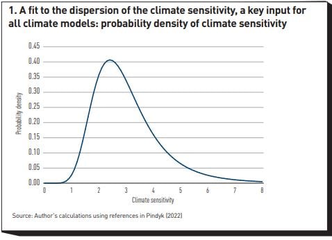
The situation is far from ideal, because economic and climate-physics models have become political tools rather than conceptual aids to make sense of what is already an extremely complex problem. In the US, a frankly outdated version of the DICE model is still used, despite the fact that (or perhaps because) it recommends very gradual abatement efforts and a low social cost of carbon. In Europe, the 1.5-2°C target has acquired totemic value, despite the fact that climate science cannot pinpoint with the degree of accuracy implied by the Paris target a ‘safe’ or ‘dangerous’ temperature range. Indeed, the best estimates of the climate sensitivity (which is a key quantity in the calibration of climate models) span as wide a range as shown in Figure 1, which displays the fit by Roe and Baker (2007)[1] to the best climate sensitivity values reported in the literature.[2] As the figure shows, there is a 10% chance that the true sensitivity may be below 1.7 or above 4.7. As the Director of the Harvard University Center for the Environment, Prof Daniel Schrag, points out, as far as we currently know there is no cliff either side of the 1.5-2°C interval. In his words, “1.5°C is not safe and 2.2°C is not the end of the world”. [3]

All of this may well be true, and an uncompromising rationalist may conclude that obsessing on this round-number target as if it were the be-all-and-end-all of climate control does not make a lot of sense. The fact, however, remains that the 1.5-2°C target has become a universally recognised policy reference point, and that it has become part of the political discourse. This has value in itself. Clear and simple targets, especially if expressible in numbers (and even more especially, if in round numbers) do serve a useful role.

This then raises the questions: can the ‘totemic’ (read, aspirational) 1.5-2°C target be reconciled with the recommendations of state-of-the-art IAMs? Can policymakers on both sides of the Atlantic re-engage with DICE-like models, or are we doomed to having differing American and European versions of climate truth?

 

How IAMs Work

To answer these questions, we must understand why the original DICE model produced such a gradual abatement schedule. As in all IAMs, there are in DICE two connected blocks. This first makes up a module that describes the world economy following the well-trodden path of Dynamics Stochastic General Equilibrium models: there are capital, labour and the total factor of production that combine via a Cobb-Douglas function to give gross economic output. To produce this output, greenhouse gases are emitted – the more so, the less the economy is ‘decarbonised’.  This is where the economic module feeds into the physics module: the industrial emissions increase the concentration of CO2 in the atmosphere, and this causes an increase in global temperature. The higher the temperature, the greater the damages inflicted on the economic output. The standard capital allocation choice (how much of the output should be saved rather than consumed) is made more complex than usual by the existence of this feedback loop from production, to temperature and to reduction in production. It is because of this feedback loop that it is rational to divert some of the productive resources to abatement initiatives. The key question is: “How much?” 

To answer this question, IAMs associate a utility with consumption, all the way from now to centuries in the future. The goal of the policy maker is then to fine-tune their ‘control variables’ (how much to save and how much to abate) so as to maximise some function of the discounted values of all these utilities.

Every single step of this procedure is fraught with uncertainties. However, some particularly deep trenches have been dug in the climate wars along a handful of key modelling points. It pays to understand why the debate is so heated, and what these bones of contention are.

The first observation is that the bulk of climate damage will be suffered by generations in the future – and, sometimes, in the very distant future. The problem therefore arises of how to ‘present value’ the utility enjoyed by future generations. Some economists (and many philosophers) have argued that we should accord to ‘future people’ exactly the same importance as we do to our contemporaries.[4] In the context of climate change, Prof Stern (2006a, 2006b) is the best-known representative in this camp, but the ‘altruistic’ tradition goes back all the way to Ramsey (1928). Most economists (Nobel laureate Prof Nordhaus amongst them) favour a ‘low’ but non-zero discount rate. The difference between Prof Stern’s 0.1% discount rate and Prof Nordhaus’ 1.5% may seem small but, given the extremely long horizons (centuries) of the climate-change problem, such small differences matter a lot. From Prof Nordhaus’ perspective, the welfare of our great-great-grandchildren has little bearing on the climate decision of a current policymaker; using Stern’s choice, future generations remain almost exactly as important as the present one. Because of this telescoping effect, the Nordhaus optimal solution envisages ‘optimal’ temperatures (and damages) for the end of the century and beyond well above the values recommended by Stern-approaches. Stern’s best abatement action is fast and in large scale; Nordhaus’ is gradual and limited in its initial scope.

Since economists and philosophers have been debating for decades (if not for centuries) the merits and blemishes of unlimited altruism, there is unfortunately little hope that this disagreement will be resolved any time soon. This is one of the two main reason why IAMs have been distrusted by policymakers.

The other main determinant of the optimal abatement policy about which there is huge disagreement is the so-called ‘damage function’.[5] For a given level of CO2 concentration, this is the function that transforms the temperature increases predicted by the climate models into damages to economic output. As Figure 1 shows, climate models may suffer from a high degree of uncertainty. However, their predictions have pin-point accuracy compared with what we can extrapolate about economic damages in response to temperature changes never experienced by human civilisation. The problem is that we have no scientific or economic theory to estimate this function, and, by and large, we have to use rather crude extrapolations. And extrapolations they must be because (fortunately) we have, so far, only observed damages for increases in global temperature of little more than 1°C, while we would like to know what might happen due to an increase of, say, 3°C or 6°C. A variety of methods have been used,[6] but there are huge variations not only across methods, but also within each method. So, for instance, for a probably very severe degree of warming of 5°C, the estimated impact on output ranges from positive 5% to negative 16%. Climate scientists have criticised economists for projecting damage values that are too low – and, indeed, in Figure 2, the red dots obtained by elicitation (mainly from climate scientists) are below the green dots estimated by econometricians for all levels of warming. However, it is not a priori clear why climate physicists should be better placed to estimate economic damages than economists. Having said this, some economists have not done themselves any credibility favours by predicting that a 5°C warming would be greatly beneficial for the planet.[7] (Should a clarification be needed, Prof Nordhaus, is not one of these overoptimistic economists.)

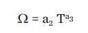
Now, the damage function used in the original DICE model belongs to the econometric class, and has been roundly criticised for being too tame. In particular, the ‘damage exponent’, ie, the quantity a3 in the equation that links temperature (T) to damages (Ω)was estimated to be equal to 2, giving rise to a relatively mild quadratic dependence of damages on temperature.[8]

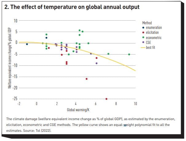
As Figure 2 shows, many different functional dependences could be estimated depending on which method is used. When used as input to an IAM, each of these different and difficult-to-justify assumptions produces very different optimal abatement schedules and carbon tax. Understandably, this has given powerful ammunition to the critics of IAMs in general, and of the DICE model in particular.

Since neither of these two sources of uncertainty is likely to be resolved any time soon, does this sound the death knell for the use of DICE-like IAMs as ‘serious’ policy applications?  Are these models destined to produce nice academic papers, or, if used in earnest, to be highjacked for political purposes? This need not be the case, because a suitably enriched version of the DICE model can provide useful guidance in navigating the stormy waters of climate policy.

 

Making IAMs Fit for Purpose

Most of the lines of criticism that have been levelled against the DICE model often use the strawman of its early incarnation, the Nordhaus (1993) version. Huge modelling strides have been made in the intervening decade. Once the DICE model is suitably enhanced, both the fundamental critiques discussed above (about the lack of agreement regarding the correct discount rate and about the damage function) lose much of their bite. Given the strength and, apparently, ‘existential’ nature of these objections, how can a perhaps-better model that still rests on such shaky foundations be of much use?  How can it escape the garbage-in-garbage-out curse? To explain how this modelling miracle is possible, we have to understand what is really wrong with the early IAM.

The original DICE model described a world with no uncertainty: the rate of growth of the population and of the economy, the damage function, the future cost of abatement with yet-to-discover technologies – everything was perfectly known to the policymaker. It was not difficult to add uncertainty and stochasticity to this or that model variable. However, when this was done, the first results were surprisingly similar to the optimal policies obtained with the deterministic version of DICE. Did the huge degree of uncertainty really not matter?

The problem was that, for computational reasons, the early IAMs invariably used what are described as constant-relative-risk-aversion, time-separable utility functions – functions , that is, that have two features: the first is that a poor and a rich agent will suffer the same pain (loss of utility) for the same percentage (not absolute) loss of wealth; the second is that today’s total welfare can be simply computed as the sum of the discounted utilities experienced at different times.

Neither of these features in isolation seems particularly unpalatable (the first one may not be empirically correct, but is certainly a big improvement over assuming absolute risk aversion). However, put together, they produce a toxic result.  The problem is that these utility functions force dislike for static risk (for taking a gamble today) and dislike for uneven consumption (which have nothing to do with each other, as the latter can arise even in a deterministic setting) to be identical. This is a big problem: if we say that we are very risk averse, we are forced to say that we strongly dislike uneven consumption. Couple this feature with the (mainstream) assumption that we shall be much richer in the future, and all of a sudden investing a lot in climate abatement becomes akin to imposing a tax on the poor (us) to benefit the rich (our great-grandchildren). The more we dislike uneven consumption, the more this ‘regressive taxation’ seems unacceptable, and the more we want to push the greatest burden of the abatement effort onto future generations. This leads inescapably to a paradoxical result for early-DICE-like models: even in the presence of huge uncertainty (say, about damages and economic growth), a high aversion to static risk causes the optimal abatement policy to be one of procrastination, not of decisive action. This is because, with the original modelling framework, the high aversion to static risk implies an equally high dislike for uneven consumption, and the two effects at best cancel each other out – at worst, they cause the optimal abatement policy to be even slower (and the carbon tax lower).

Is there really no way out of the impasse? There certainly is: if we use so-called recursive utility functions (e.g., of the Epstein and Zinn, 1989 class), we can assign independently a coefficient of aversion to static risk, and a coefficient of aversion to uneven consumption. With a realistically strong dislike for static risk,[9] the great uncertainty about climate outcome can now have the expected effect of making the abatement strategy prompter and more decisive, without the dislike for uneven consumption (that can be parametrised independently) working in the opposite direction.

Seen in this light, the extremely high uncertainty about climate damages (and, to a lesser extent, about the physics of the problem) no longer render IAMs useless: knowing that we don’t know, and knowing how ignorant we are, immediately makes the optimal policy more prudent, the abatement effort more urgent, and the carbon tax higher.

Why did the early IAMs make use of the time-separable power utility functions? Why weren’t aversion to static risk and to uneven consumption decoupled from the start? Because recursive utility functions, which allow the independent parameterisation of these different ‘preferences’, are indeed much more palatable (every economist agrees on this), but come at a high (and, until recently, exorbitant) computational cost. Luckily, more powerful computers, but, above all, smart computational techniques–including some spearheaded by EDHEC-Risk Climate Impact Institute–have turned a near-impossible task into a reasonably manageable one.     

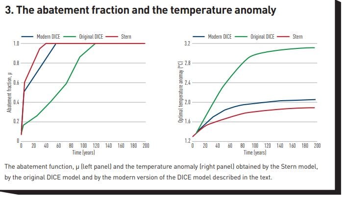
What about the ‘philosophical’ debate about how altruistic we should be towards future generations – about, that is, the rate of utility discounting? No degree of computational wizardry can solve what is in essence an ethical problem. However, when the aversion to static risk and to uneven consumption are disentangled, and a realistic degree of uncertainty is injected in the problem, the optimal abatement schedule produced by the new-and-improved DICE model with the same degree of impatience posited by the original DICE model is already so ambitious and aggressive (and the carbon tax so high), that it is already at the limit of what is practically and politically achievable. In practical terms, once we disentangle aversion to static risk and uneven consumption with recursive utility functions, we no longer need to be infinitely (and, arguably, unrealistically) altruistic to obtain an optimal solution close to Stern’s extremely aggressive recommendations. See in this respect the left panel of Figure 3, which also shows in the right panel the similarity of the optimal temperature profile recommended by the Stern and the `modern DICE’ approach, and the much higher optimal temperature obtained by the original DICE model.

It is also important to stress that the modern-DICE optimal temperature remains within the Paris accord 1.5-2°C target by the end of the century – it is in this sense that the staying within the target can be justified as an optimal policy, and not just an ‘aspiration’. For the reasons discussed in the opening paragraphs, the importance of this result should not be underestimated.[10]  

 

 

From Optimality to Implementation

Knowing what would be optimal to do is clearly important, and it is good to know that an abatement schedule that keeps the temperature between 1.5°C and 2°C by the end of the century is, in principle, technologically achievable, especially if carbon removal is allowed (see in this respect the discussion in footnote 10). The magnitude of the task, however, should not be underestimated. Figure 4 shows the historical CO2 emissions from 1850 to date in the left part of the graph, and, in its right portion, the optimal emission path obtained by the modern DICE approach – a path that, let’s remember, just keeps us inside the Paris Agreement target.  

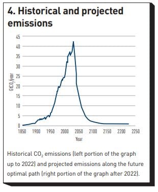
Clearly, an unprecedented change in the global emission policy must take place, and the required change of abatement pace is, literally, breath-taking. Has anything similar been so far been observed?[11] Yes and no. Figure 5 (left panel) shows the per capita CO2 emissions in France from the start of the nineteenth century to date. If we neglect the dips associated with the two world wars (this is not how we want to curb emissions), we note a remarkably sharp fall in emissions starting in the late 1970s.  

 

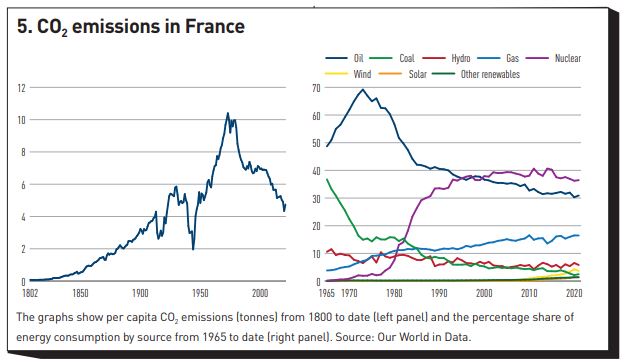
The drop is clearly attributable to the peculiarly French choice of adopting nuclear energy as its dominant energy source: notice, from the right panel the parallel drop in oil, brusquely reversing what had been a steady increase until the late 1970s.

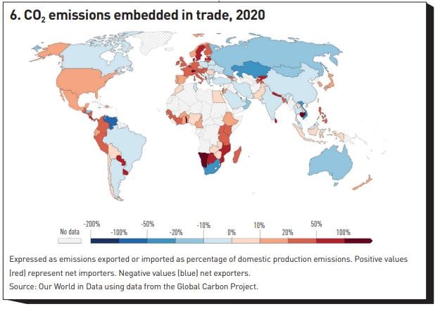
Now, the most pronounced drops in CO2 emissions per capita to date have occurred in the Western world and, as far as we have been able to ascertain, in no major country have the drops been faster than in France[12]. Since few countries share the same enthusiasm as France for nuclear energy, it is difficult to see this pace of abatement repeated elsewhere.[13] In Germany, for instance, despite its enthusiastic embrace of sources of renewable energy, the pace of abatement has been 50% slower than in France. And, in any case, even looking at how quickly the ‘best in class’ have managed to abate can be seriously misleading. As Figure 6 shows, all European countries have ‘exported’ a significant part of their emissions (by having parts of the goods they consume manufactured elsewhere – often in parts of the world with lower emission standards). When imported emissions are taken into account, China has grown emissions some 10% less than its headline figure, but, depending on the country, European emission figures should be increased by up to 68% (for Sweden).

 

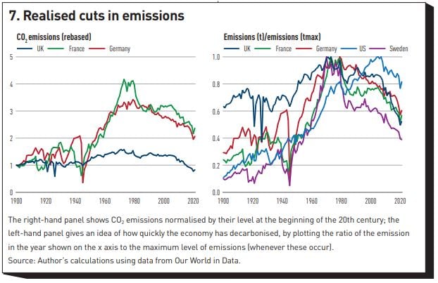
The realised declines in emissions are shown in Figure 7 for a handful of countries, each representative of different approaches to apparently successful abatement: the right-hand panel shows the CO2 emissions normalised by their level at the beginning of the twentieth century; the left-hand panel then gives an idea how quickly the economy has decarbonised, by plotting the ratio of the emissions in the year shown on the x axis to the maximum level of emissions (whenever these occur). We note first for all countries the maximum emissions are reached around the mid-to-late 1970s. We have discussed the case of France and Germany. Sweden seems to have achieved a relatively impressive feat of emission reduction. However, the imported emission have grown steadily for Sweden from 48.6% in 1990 to 68.5% in 2020. When this figure is factored back in, the Swedish emission decreases from peak are much less impressive. The UK also seems to have achieved a very significant reduction in emissions from peak, but the left-hand panel shows a very atypical pattern for Western countries because in the 1960s and1970s the increase in emission was much more muted. And, in any case, the ‘hidden’ emissions coming from trade have steadily grown for the UK from 11% in 1990 to 42% in 2020 (the same figures are 13% to 20% for Germany, with the initial low figures distorted by the German unification).

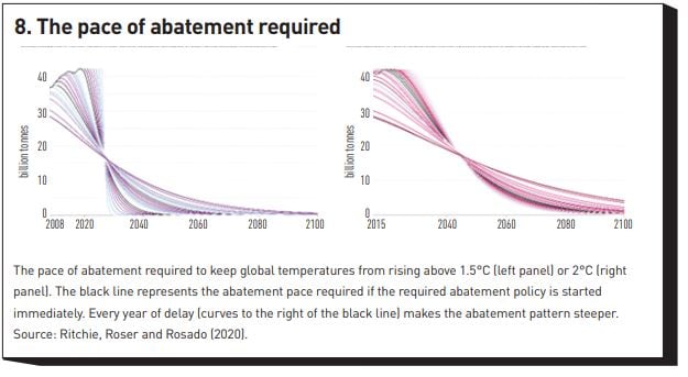
So, this is what the best in class have managed to achieve in terms of pace of decarbonisation. In the light of this, how difficult is it really to meet the Paris Agreement temperature ambitions? Figure 8, which displays the pace of abatement required to remain within 1.5°C (left panel) and 2°C (right panel) suggests an answer. Without negative emissions, the more ambitious goal is essentially unattainable; and the 2°C target requires sustained reductions in (trade-adjusted) emissions the like of which has not been seen anywhere in the world – and, when it has been approximated, the feat has been achieved only thanks to a massive switch to nuclear energy.  To put things in perspective, the unique, nuclear-energy-led fall in emissions experienced in France has seen a reduction of 53% in 28 years; the required global fall in emissions to remain within the less ambitious target of 2°C by the end of the century requires approximately the same percentage reduction in 22 years – and this is before correcting for trade-embedded emissions.

Of great concern is also the fact, while the production of energy from renewables has doubled in the last decade, global emission have also increased and this is mainly due to emission-intensive sources (such as the production of cement or steel), for which there are currently very few large-scale non-fossil-fuel alternatives.[14] The key problem is that the appetite for cement and steel seems insatiable: Smil (2022) reports that in the two pre-Covid years China alone produced roughly as much cement (4.4 bn tonnes) as the US during the whole of the twentieth century. Unfortunately currently “there are no large-scale, proven ways of producing these four material pillars [cement, steel, plastic and ammonia] of modern civilisation with electric energy alone (green or otherwise)” (Rebonato, 2023).

 

 

What Does This Mean for Investors?

This paper has described in very broad terms what the latest-generation IAMs tell us about the optimal course of climate action, and how achievable this target may be. A lot more could be said on topic – the most glaring omission being the important role that negative emissions must play in any realistic 1.5-2°C strategy. [15] A few key messages stand out:

• when updated to reflect the latest advances in physics and economics modelling, IAMs can give very useful policy advice;
• the recommendations they provide point to a much faster and steeper abatement policy than the original DICE model indicated – a policy consistent with the 1.5-2°C Paris target;
• this fast abatement pace is technically possible, but (apart from what observed during World Wars) it would be unprecedented: technologically not impossible, but by no means a ‘central scenario’.

What does mean for investors? Which abatement scenarios are current asset prices reflecting? Are substantial price adjustments to be expected?

Answering these questions is far from easy, because it has proven difficult to establish to what extent asset prices have moved so far in response to climate news. The very fact that detecting the impact of climate risk on prices has proven so difficult, however, points to the fact that the price sensitivity so far cannot have been very pronounced. Let’s assume that this is true – that asset prices, that is, have to date changed relatively little because of our climate predicament. This could mean three things:

• that the market believes that, whatever the climate outcome, the impact on asset prices will be very limited;
• that the market believes that ‘this time is different’ and all the major emitters will stick to their pledges, and actually increase them, and the temperature increases will be contained (possibly within the Paris Agreement target);
• that the market is ‘asleep at the wheel’.

The first option (the irrelevance of a poorly controlled climate outcome for asset prices) is difficult to believe. Perhaps it is true that the economic (certainly not the human!) cost, as such cost is currently measured, will be limited, but clearly, we cannot be sure of this. See Pindyck (2022) in this respect. And in any case, as we have seen, just our uncertainty about the economic effects should affect asset prices. As we hear after every election with an unclear outcome, “Markets hate uncertainty’. If the first explanation is true, this time they seem, if not to love it, at least to ignore it.

The second possibility requires a very high degree of confidence in an unprecedented change in actual climate action (without cosmetic adjustments behind the smoke screens of exported emissions). As Pyndick (2022) points out, every major climate pledge to date has been broken or ‘massaged to hit the numbers’. And even if the currently pledged reductions were enacted, they would still fall somewhat short of the 2°C (let alone a 1.5°C) target.  

The third possibility (that the market is currently wearing climate blinkers) is in my view the most likely, buy clearly flies in the face of any notion of market efficiency. If markets were to adjust their expectations of the impact of climate change on cashflows and profitability in a sudden and disorderly fashion, this could create sudden asset repricing and heightened volatility.  

It is difficult at the moment to state with confidence which of the three possibilities is the correct one. All of this, however, points clearly to two topics for further investigation: first, measuring what the impact on asset prices of different climate outcomes can be (see in this respect preliminary work by Rebonato, Kainth and Melin (2023)); and, second, assessing to what extent this information is reflected in prices. Both these pieces of information are necessary to establish a connection between economic modelling, actual climate policy, and the impact of this on asset prices. Research in both these directions is under way at EDHEC-Risk Climate Impact Institute.  

 

Footnotes

[1] For a good discussion, see Pindyck (2022).

[2] Climate sensitivity is the rise in global temperature in response to a doubling of CO2 concentration with respect to pre-industrial levels. It is a key input to all climate models.

[3] Professor Daniel Schrag quoted in The Economist, November 2022. Available at: https://www.economist.com/interactive/briefing/2022/11/05/the-world-is-going-to-miss-the-totemic-1-5c-climate-target. 

[4] See, e.g., Sidgwick (1907), Harrod (1948), Solow (1974), Dasgupta (2020).

[5] The rate of growth of the economy also has a very large effect on the optimal solution. There is, however, much less disagreement among economist about this quantity. If we are sure that our grandchildren will be much richer than we are, engaging in large and costly abatement today would be akin to imposing a tax on the poor (us) to benefit the rich (our grandchildren). How much we dislike uneven consumption plays an important role in determining how important this consideration is.  

[6] Kainth (2022) distinguishes the enumeration, elicitation, econometric and Computational General Equilibrium approach, and discusses the strengths (few) and weaknesses (many) of each.

[7] Among the ‘optimistic’ results, the work by UCSB Professor Olivier Deschenes (2007, 2011) should be mentioned. One of the arguments of those economists who predict a net benefit from global warming is that the increase of CO2 in the atmosphere will enhance the growth of agricultural foodstuff (the so-called ‘CO2 fertilisation effect’.)

[8] A damage exponent of approximately 2°C (1.98) was independently estimated by Rudik (2020). In theory, there is a linear term in a1 but, when a quadratic term is present, this coefficient is usually estimated to be zero.

[9] I say `realistically’ because all estimates of the coefficient of relative risk aversion from observed asset prices point to values much higher than the 1.45 posited in the DICE model. In their seminal paper, Bansal and Yaron (2004) estimate a coefficient of aversion to static risk above 10.

[10] Research carried out at EDHEC-Risk Climate (Rebonato, Kainth, Melin and O’Kane, 2023) extends this analysis to the case when negative emission technologies are available alongside traditional abatement tools. A detailed discussion would take too long a detour, but the qualitative results are not changed. If anything, the optimal temperature path is a bit lower than shown in the second panel of Figure 3. 

[11] The analysis that follows is based on data made available by the excellent resource Our World in Data. 

[12] This is after adjusting for ‘exported emissions’ – see the discussion to follow.

[13] Higher safety standards and a loss of engineering expertise due to reduced building activities in the last decades may also limit the speed at which one can develop the share of nuclear power in the next decade.

[14] Source: McKinsey Report, “The energy Transition: A Region-by-Region Agenda for Near-Term Action”, December 2022. See also Smil (2021).

[15] See, in this respect, the EDHEC-Risk Climate Impact Institute paper by Rebonato, Kainth, Melin and O’Kane (2023).

 

References

Bansal, R., and A. Yaron (2004) Risks for The Long Run: A Potential Resolution of Asset Pricing Puzzles, Journal of Finance 59(4): 1481-1509.

Dasgupta, P. (2020) Ramsey and Intergenerational Welfare Economics, The Stanford Encyclopedia of Philosophy (Summer Edition), E.N. Zalta (Ed.). Available at: https://plato.stanford.edu/archives/sum2020/entries/ramsey-economics/

Deschênes, O., and M. Greenstone (2007). The economic impacts of climate change: evidence from agricultural output and random fluctuations in weather. American Economic Review 97(1): 354-385

Deschênes, O., and M. Greenstone (2011). Climate change, mortality, and adaptation: Evidence from annual fluctuations in weather in the US. American Economic Journal: Applied Economics 3(4): 152-185.

Epstein, L.G., and S.E. Zin (1989) Substitution, Risk Aversion, and the Temporal Behavior of Consumption and Asset Returns: A Theoretical Framework, Econometrica 57 (4): 937–969

Harrod, R.F. (1948) Towards a Dynamic Economics, Macmillan, London.

Kainth, D. (2022) Recalibrating the DICE Climate Model, EDHEC-Risk Climate technical report, 1-22.

Nordhaus, W. (1993) Rolling the `DICE': An Optimal Transition Path for Controlling Greenhouse Gases, Resource Energy Economics 15: 27-50.

Pindyck, R.S. (2022) Climate Future – Averting and Adapting to Climate Change, Oxford University Press, Oxford, UK.

Ramsey, F.P. (1928) A Mathematical Theory of Saving, Economic Journal, December: 57-72.

Rebonato, R. (2023) How to Think About Climate Change – Insights from Economics for the Perplexed but Open-Minded Citizen. Cambridge University Press, forthcoming.

Rebonato, R., D. Kainth, and L. Melin (2023) Climate Output at Risk, Journal of Portfolio Management 49(2): 10.3905/jpm.2022.1.414.

Rebonato, R., D. Kainth, L. Melin and D. O’Kane (2023) Optimal Climate Policy with Negative Emissions, EDHEC-Risk Climate working paper. Available at: https://papers.ssrn.com/sol3/papers.cfm?abstract_id=4316059.

Ritchie, H. M. Roser, and P. Rosado (2020) CO₂ and Greenhouse Gas Emissions. Our World in Data. Available at: https://ourworldindata.org/co2-and-other-greenhouse-gas-emissions.

Roe, G.H., and M.B. Baker (2007) Why Is Climate Sensitivity So Unpredictable? Science 318: 629-632.

Rudik, I. (2020). Optimal Climate Policy When Damages Are Unknown. American Economic Journal: Economic Policy 12(2): 340-73).

Sidgwick, H. (1907) The Methods of Ethics, MacMillan, London, 7th edition.

Smil, V. (2021) Grand Transitions: How the Modern World Was Made, Oxford University Press, Oxford, UK.

Smil, V. (2022) How the World Works: A Scientist's Guide to Our Past, Present and Future, Viking Press, NY.

Solow, R.M. (1974) Intergenerational Equity and Exhaustible Resources, Review of Economic Studies 41: 9-45.

Stern, N. (2006a) The Economics of Climate Change – The Stern Review”. Technical report, HM Treasury, UK, HM Treasury.

Stern Review (2006b) The Stern Review on the Economic Effects of Climate Change, Population and Development Review 32(4): 793-798.

Tol, R.S.J. (2022). A meta-analysis of the total economic impact of climate change. CESifo Working Paper, No. 9919. Available here: https://www.cesifo.org/en/publications/2022/working-paper/meta-analysis-totaleconomic-impact-climate-change