Why We Need Climate Scenario Probabilities and How to Get Them

This article by Riccardo Rebonato, Scientfic Director of EDHEC-Risk Climate, has been originally published in the December 2024 newsletter of the Institute. To subscribe to this complimentary newsletter, please contact: [email protected].

1. Why We Need Climate-Scenario Probabilities

When investors and policymakers are faced with the garden-variety uncertainty associated with financial quantities, they have at their disposal well-established statistical tools, such as Value-at-Risk or Expected Shortfall (see, eg, McNeil, Frey, and Embrechts (2015)). Knowing that there are more things between heaven and earth that are dreamt of in the statisticians’ philosophy, the same investors and policymakers often also make use of scenario analysis. The two approaches complement themselves: as the slogan goes, statistical tools are backward-looking and scenarios (can be) forward-looking.

Financial scenarios are rarely, if ever, accompanied by explicit probabilities. However, the ‘expert knowledge’ of the end users allows them to understand whether a given scenario represent a clear and present danger, or whether it belongs to the meteorite-falling-on-Earth category. And, if they so wanted, the same users could avail themselves of a hundred-year-plus of financial data to carry out a formal assessment of the scenario likelihood. So, with financial scenarios, probabilities are at least in the back of the users’ mind, and can be brought centre stage with relatively little effort.

Climate scenarios are different. Since the effects of climate change on the real economy and on financial assets are only just beginning to become apparent, a ‘climate Value-at-Risk’ based on experienced losses is hardly feasible, closing the backward-looking route to climate-risk assessment. Scenarios understood as the contemplation of yet-never-experienced climate outcomes therefore become particularly important. However, the expert knowledge of the same scenario users is of little help in gauging the likelihood of different climate futures. Any portfolio manager worth her salt should have an opinion on the severity of a scenario such as ‘a parallel move in yields by 100 basis points’. How confident would the same portfolio manager be to opine about the relative likelihood of a 4.5 versus an 8.5 end-of-century forcing – assuming, that is, that she understands what that means?

Leaving more of less extreme outcomes to one side, investors sorely need a probabilistic dimension to climate analysis. As Finance 101 teaches, prices are the sum of discounted expected cashflow. The ‘expected’ bit in the valuation slogan means that we need probabilities in order to value securities: it is not enough to know what can happen, and how to discount these future cashflows; we also need to have an idea of how likely the different cashflows will be. So, without a probabilistic dimension the whole valuation project grinds to a halt.

This state of probabilistic confusion is not confined to investors. The Intergovernmental Panel on Climate Change has produced several carbon pathways of different severity (with the severity expressed as radiative forcing, ie, the imbalance between energy in and energy out). The same body, however, has not provided any probabilistic guidance as to how ‘seriously’ the various forcings should be taken. In their research (see, eg, Burke, Hsiang, and Miguel (2015) an Kotz, Leverman, and Wenz (2024)) climate scientists and economists have predominantly made use of the severest pathway (the so-called RCP8.5). Despite this profligate expenditure of analytical resources, Hausfather and Peters (2020) has argued that this scenario should be never considered, because virtually impossible (Schwalm, Glendon, and Duffy (2020), by the way, disagrees). Are they correct? Without some form of probabilistic framework, we cannot tell. If we do not want to be condemned to the fate of the drunkard in the night who looks for his keys under the lamppost because that is where light is, we need some probabilistic indication of where we should focus our analytical gaze.

Having probabilities for climate outcomes would be nice, it is often claimed, but it is well-nigh impossible. We may be able to say something meaningful about the uncertainty in economic growth, in the climate physics, or in the function that translates temperature increases into damages. But, the prevailing argument goes, policy uncertainty is so intractable as to kill the probabilistic project in the bud. We agree that policy uncertainty is indeed the most difficult aspect of the problem to model; and we also agree that we will never arrive at ‘sharp’, two-decimal-places probabilities. What we want to show is that the idea that we cannot compare the likelihood of different abatement policies because of irreducible uncertainty is overly pessimistic. While it is true that some outcomes are uncertain and hard to predict, we believe it is possible to make informed assessments and weigh the probabilities of different outcomes based on the evidence we have. We therefore intend to propose two avenues to arrive at imprecise but actionable probabilistic statements about future climate outcomes.

2. Two Routes to Policy Probabilities

How aggressive can an abatement policy be? Can we ‘quantify aggressiveness’? Abatement policies are obviously bounded from below by the strategy of doing (close to) nothing. However, there are also upper bounds to how quickly the economy can decarbonize. The limits are technological (how many, say, wind turbines can be produced in a year), but also fiscal/monetary. Much as we like to wax lyrical about the green dividends of the decarbonization of the economy, any serious modelling approach shows that a part of net economic output must be diverted from consumption and investment to costly abatement. Pre-climate-change economic agents only had to choose how much of the GDP to consume and how much to save to produce greater future consumption. Post-climate-change agents are faced with a more difficult choice, because the tomorrow’s greater consumption, if obtained by burning fossil fuel, will reduce the day-after-tomorrow’s consumption because of climate damages. How great is the optimal diversion of resources to costly abatement (how aggressive, that is, can we expect the abatement policy to be)? Ultimately this is the vexed size-of-carbon-tax question. We can’t know for sure, but we can have some indications.

A carbon tax of 100% of GDP is obviously a hard bound. But, in practice, we can find much tighter constraints. Globally, we spend approximately 3% of GDP on education and defence. Healthcare absorbs between 8-to-10% of world GDP. It is difficult to imagine that a much greater fraction of GDP would be devoted to climate control. To give an example, Russia is at the moment devoting about 8% to its war machine, and, by so doing, greatly distorting its economy (with rampant inflation, a weakening currency and unemployment just above 2%). And even in darkest hours of World War 2 no country devoted more than 40% to military expenditure. We can therefore start by imposing soft bounds that become more and more binding as we exceed the amount of GDP devoted to healthcare and we move towards the theoretical limit of 100% of GDP. So, if we take the social cost of carbon (‘carbon tax’) as a reasonable proxy for the abatement aggressiveness, we already know that its probability distribution should begin falling pretty quickly as we exceed that healthcare-expenditure level, and go to zero when we reach 100% of GDP.

Is there anything else that we can say? The European market for CO₂ emission permits has been active for more than 20 years and has now entered a mature phase. If we equate the observable cost of a permit with a carbon tax, we can say that the expectation (the average value) of the possible carbon taxes should be equal to the observed cost of a permit. When we do so, we have bounded the distribution, and we have specified its fist moment. Can we bring more information to bear on the shape of the distribution ? It depends on what we mean by ‘information’. If we ask for direct information, the answer is ‘probably no’. If this is our answer, then we are embarking on the route that will take us to our first approach to probability estimation. There can be, however, some additional information – no doubt, imperfect and partial, but information nonetheless. It is to be found in the expert opinion of professional economists about the optimal social cost of carbon. This information will have to be curated and bias-corrected, but, once we do so, will lead to the second path to our probability estimates.

If we take the first approach, we are embracing the so-called least-committal (maximumentropy) approach. This method has solid theoretical foundation, being rooted as it is in the pioneering work in information theory by Shannon (1948). Beyond the theoretical appeal of the model, it is the range of successful practical applications, in fields as diverse as biological systems (see, eg, DeMartino and DeMartino (2018)), natural language processing (see, eg, Berger, DellaPietra, and DellaPietra (1996)) or statistical physics (see, eg, Jaynes (1957)), that has made it the go-to probabilistic model when one wants to use in the most effective way what one does know about a system, without adding any unwarranted information.

If we take instead the second approach, then our task will be to make the distribution of expert opinion elicited from economists consistent with our bounds, and to correct it for what we call the politician-economists bias (the fact, that is, that, unlike politicians, economists do not face re-election). We briefly present the two approaches below. What is reassuring is that, despite the seemingly very different starting points, the probabilistic projections they produce turn out to be very similar.

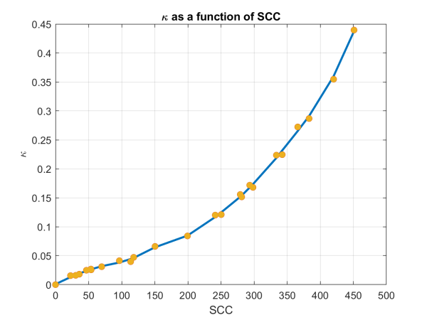
In both cases, our proximate goal is a probability distribution for different values of the carbon tax. This is close to, but not quite, what we need: a probability for policy aggressiveness. To make this last step we use a surprisingly robust empirical result: if we characterize the abatement policy by an effective abatement speed (roughly, by how much, in percentage terms, we reduce emissions per year), we can show that there is a strong (monotonic) relationship between the optimal social cost of carbon and the abatement speed, as shown in Figure 1.

Thanks to this one-to-one correspondence between the social cost of carbon and the policy aggressiveness, if we have a probability distribution for the former we can easily find the distribution for the latter. We therefore focus in what follows on how to find the distribution for the social cost of carbon. 

Figure 1: The abatement speed, κ1 (years−1, y axis) as a function of the optimal social cost of carbon ($/ton CO₂, x axis).

The continuous curve is a LOWESS (Cleveland (1979)) quadratic smooth fit to the calculated points, shown as filled yellow dots.

2.1 The Least-Committal Distribution
 

If we follow to the maximum-entropy route to solving this problem, a straightforward application of functional calculus gives for the social cost of carbon, x, the following (exponential) distribution:

ϕ(x) = K exp(−λ · x)                                                                                                  (1)

with K and λ derived in Rebonato (2025). So, according to this solution, the probability a given carbon tax decreases as the tax increases – a reasonable enough behaviour given
common voters’ preferences.

2.2 The Informative (Economists’) Distribution
 

With the second approach, we say that we actually know something more than ‘voters don’t like taxes’, and that the expert opinion about how much we should spend to contain climate change does have some bearing on voters’ choice. Note that we are adding information – that we ‘claim to know more’ – and, as a result, the distribution we obtain will be different from the maximum-entropy distribution.

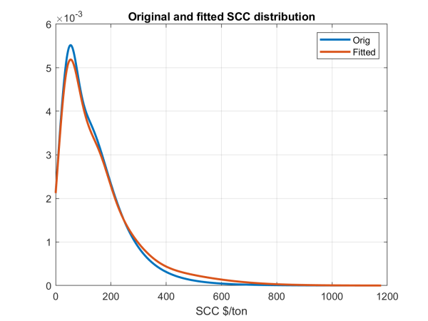
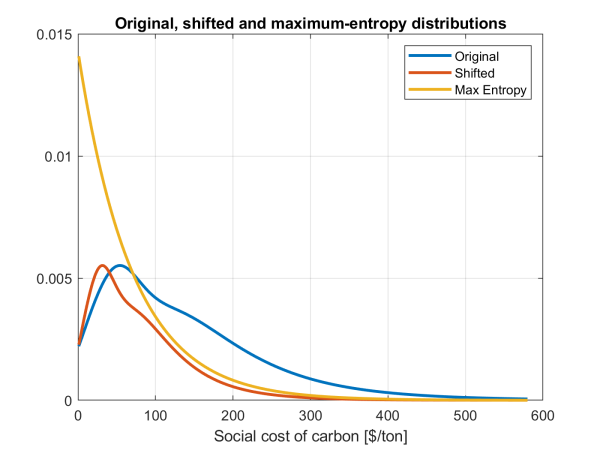
As mentioned, economists do not face the same incentives as politicians do, and their opinions will therefore be biased (upwards, towards more aggressive distributions). Furthermore, they do not always take into account the ‘soft constraints’ we have mentioned above. This means that the distribution of their opinion must be curated in a variety of ways, as described in detail in Rebonato (2025). When this exercise in data curation is carried out, we arrive at the distributions shown in Figure 2 (one curve shows the empirical distribution and the other the fit obtained using a mixture of truncated Gaussian and lognormal distributions). For comparison Figure 3 then shows the maximum-entropy distribution (yellow line); the non-bias corrected economists’ distribution (red line) and the corrected (shifted) economists’ distribution (blue line).

Figure 2: The fit to the empirical distribution obtained using a mixture of a truncated Gaussian

and a lognormal distribution. Social cost of carbon in 2010 USD on the x axis.

We have presented our approach with a very broad brush, and we have omitted many important details (again, see Rebonato (2025) for a fuller description). We are, however, already in a position to discuss some interesting results.
 

Figure 3: The original (red line), shifted (blue line) and maximum-entropy (yellow line) distributions. Social cost of carbon in 2010 USD on the x axis.

3. Results

When it comes to economic and financial applications, the assumption is almost universally made that temperature increases (the so-called ‘temperature anomalies’) are a powerful statistic of impairment to GDP (see, eg, the seminal studies by Burke, Hsiang, and Miguel (2015) and Kotz, Leverman, and Wenz (2024)). There still is little consensus about the correct mapping from temperature to damages (and our research group are engaged at the forefront of this exciting topic); for the purpose of this analysis we therefore limit our analysis to assigning probabilities to temperature outcomes. We choose the end of the century as our reference horizon.

Before presenting our results, we must make clear that the final temperature distribution will depend not only on the distribution of abatement speeds, but also on our assumptions about economic and demographic growth, and about climate uncertainty. We document our choices for these quantities in Rebonato (2025), but we stress that our original contribution is in how to deal with the ‘intractable’ (ie, the policy) part of the problem. In this respect, our contribution is non-policy-model agnostic, and transportable to different scenario engines.

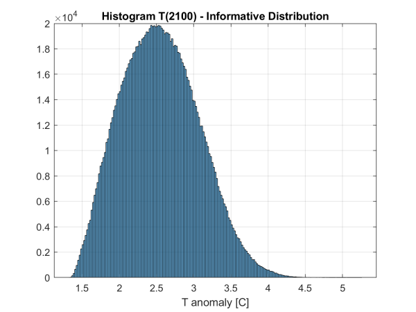
In a typical configuration, we find the temperature distribution shown in Figure 4. The first observation is that the likelihood of limiting end-of-century temperature increases to 1.5°C is very small: the exact value depends on the modelling choices, but these probabilities are never larger than a few percentage points. We stress that the goal is technologically achievable, but it would require a major and sudden alignment of actual abatement policy with the consensus (median) recommendations of economists. Since economists have put forth these abatement recommendations for the best part of half a century, and their suggestions have gone largely unheeded, our method finds that the probability of an imminent correction of the politician/economist disconnect is highly unlikely. Since the highest transition (abatement) costs are associated with the achievement of the 1.5°C target, this has direct asset valuation implications, as it gives low weight to the most ‘costly’ abatement paths.

Next, we find that the median 2100-temperature anomaly (around 2.5°C) is well above the 2.0°C end-of-century target, and that there is a significant probability (around 35-40%) that the temperature will exceed 3°C (again, its precise value depends on the specific modelling choices, but, no matter which reasonable model configuration we choose, it is never less than 20%). To put these figures in perspective, the human species, let alone civilization, has never experienced temperature anomalies of 3°C or higher. Such high temperatures would push us into uncharted territory, increasing the likelihood of tipping points—sudden and potentially irreversible climate shifts triggered by crossing critical thresholds. These events, while difficult to predict, would severely challenge adaptation efforts and lead to significant physical damages. In any case, the large probability mass that we estimate for relatively high temperatures suggests that physical damages are likely to be greater than transition costs. Another way to look at our results is that our estimates assign low probabilities to high-transition-cost scenarios.

The distribution in Figure 4 was obtained using the ‘informative’ approach. How different would our conclusions be if we had used the maximum-entropy approach? How robust, in other words, are our results? We find that the expected 2100 temperature anomalies obtained with the politicians’ and the maximum-entropy distributions are very similar (2.75°C and 2.80°C for the elicited and maximum-entropy distributions, respectively). All the temperature percentiles obtained using the maximum-entropy distribution are higher, but the differences are always small. And it is easy to understand why the economists’ distribution gives rise to somewhat smaller temperatures: if we take the economists’ views into account we add the information that extremely low abatement speed should be unlikely (see again Figure 3), and this marginally reduces the terminal temperature.

Figure 4: Histogram of the 2100 temperature anomaly for a typical configuration (informative distribution, shift m = 50).

4. Conclusions

These are sobering results. If our analysis is correct, the likelihood of a relatively safe ‘climate landing’ is small – much lower than the probability of ending up with unprecedentedly high, and probably very dangerous, temperature increases. What would it take to change the probabilities of these outcomes?

There has been no dearth of dire warnings about the dangers of poorly controlled climate change. What has been lacking has been a link between this expert knowledge and the actually implemented policies – this, after all, is at the origin of the shift in the economists’ distribution, and of the centring of the maximum-entropy distribution that play such an important part in our approach. The shift is large, and it is due to the fact that the actual carbon tax (or, rather, its proxy, the cost of emission permits) is still very far from what the economists recommend it should be. In simple terms, we are not diverting enough of our disposable income towards climate abatement to buy for ourselves and our children a meaningful amount of climate insurance. As long as this remains the case, both the economists’ and the maximum entropy distributions will remain shifted towards the little-abatement end of the spectrum.

One can quibble with the precise quantification of the probabilities we arrive at – probabilities that, in any case, are not at all intended to be sharp. However, unless there is a major shift in our willingness to fund, via costly abatement, the green transition, the mass of the probability distribution will remain shifted towards the low-abatement end of the axis. The temperature distribution we show in Figure 4 should give investors, policymakers, and citizens in general, food for climate thought.

Acknowledgments: It is a pleasure to acknowledge substantial contributions to this work offered by Dr D. Kainth (who is also specifically acknowledged in the text). Thanks are also due to Dr L. Melin, Dr F. Zhang and Mr F. Ducoulombier. 

References:

• Berger, A. L., S. A. DellaPietra, and V. J. DellaPietra (1996): “A Maximum Entropy Approach to Natural Language Processing,” Computational Linguistics, 22(1), 39–71.
• Burke, M., S. Hsiang, and E. Miguel (2015): “Global Non-linear Effect of Temperature on Economic Production,” Nature, 527(7577), 235–239.
• Cleveland, W. S. (1979): “Robust Locally Weighted Regression and Smoothing Scatterplots,” Journal of the American Statistical Association, 74(368), 829–836.
• DeMartino, A., and D. DeMartino (2018): “An Introduction to the Maximum Entropy Approach and Its Application to Inference Problems in Biology,” National Library of Medicine, doi: 10.1016/j.heliyon.2018.e00596.
• Hausfather, G., and G. P. Peters (2020): “Emissions – The ‘Business as Usual’ Story is Misleading,” Nature, 577, 618–620.
• Jaynes, E. T. (1957): “Information Theory and Statistical Mechanics,” The Physical Review, 106(4), 620–630.
• Kotz, M., A. Leverman, and L. Wenz (2024): “The Economic Commitment of Climate Change,” Nature, 628, 551–557.
• McNeil, A. J., R. Frey, and P. Embrechts (2015): Qunatitative Risk Management. Princeton University Press.
• Rebonato, R. (2025): “How to Assign Probabilities to Climate Scenarios,” EDHEC-Risk Climate Working Paper, pp. 1–69.
• Schwalm, C. R., S. Glendon, and P. B. Duffy (2020): “RCP8.5 Tracks Cumulative CO2 Emissions”,” PNAS, 117 (33), 19656–19657. 
• Shannon, C. E. (1948): “A Mathematical Theory of Information,” Bell System Technology Journal, 27, 379–423.